Representability

A question that asks for its own space

Mathematics often begins a classification by making a set: lines in the plane, divisors on a curve, closed subschemes of projective space with a fixed numerical profile, or varieties of a chosen kind. The geometric problem is whether its members vary algebraically, nearby parameters describe nearby objects, and one universal family has the classified object as each fiber.

Grothendieck’s representability method changed the order. Before trying to topologize a set of answers, define how answers vary over every base. To each test scheme $T$, assign the set of families over $T$. Make this assignment functorial under base change. Then ask whether there is a scheme $M$ such that maps $T\to M$ correspond naturally to those families. If so, $M$ represents the functor.11Grothendieck and Dieudonné, “Éléments de géométrie algébrique III: Étude cohomologique des faisceaux cohérents, première partie”; Grothendieck, “Technique de descente et théorèmes d’existence en géométrie algébrique. II. Le théorème d’existence en théorie formelle des modules”.

The change is easy to state and difficult to fulfill. A set of isomorphism classes can exist while no scheme represents the family functor. Automorphisms can prevent a universal family. Quotients can fail. Flatness and boundedness can be missing. The method is powerful because it turns “the parameter space should exist” into a theorem with exact content and possible failure.

The documentary trail is unusually sharp. Grothendieck’s letter to Jean-Pierre Serre dated October 31, 1959, links descent techniques and formal geometry to the characterization of functors

$$T\longmapsto\operatorname{Hom}_S(T,X).$$

He was working toward a general existence theorem in scheme theory while Dieudonné moved early EGA chapters through the press. Four months later, in February 1960, Grothendieck’s Bourbaki exposé opened by defining representable and pro-representable functors.22Grothendieck and Serre, Correspondance Grothendieck–Serre, 101; Grothendieck, “Technique de descente et théorèmes d’existence en géométrie algébrique. II. Le théorème d’existence en théorie formelle des modules,” 369.

Classification that varies

Consider lines in the projective plane. A line with coefficients $[a:b:c]$ has equation33Grothendieck and Dieudonné, “Éléments de géométrie algébrique III: Étude cohomologique des faisceaux cohérents, première partie”; Grothendieck, “Technique de descente et théorèmes d’existence en géométrie algébrique. II. Le théorème d’existence en théorie formelle des modules”.

$$ax+by+cz=0,$$

where simultaneous scaling does not change the line. The lines are therefore parameterized by a dual projective plane. This familiar example contains the pattern: a parameter point determines an object, and there is one incidence subvariety44Grothendieck and Dieudonné, “Éléments de géométrie algébrique III: Étude cohomologique des faisceaux cohérents, première partie”; Grothendieck, “Technique de descente et théorèmes d’existence en géométrie algébrique. II. Le théorème d’existence en théorie formelle des modules”.

$$\mathcal L\subseteq(\mathbb P^2)^\vee\times\mathbb P^2$$

whose fiber over $[a:b:c]$ is the corresponding line.

But field-valued points are only the first layer. Let the coefficients vary over a scheme $T$. A $T$-family of lines should correspond to a map $T\to(\mathbb P^2)^\vee$, subject to the correct line-bundle formulation. Pulling the incidence family back along that map gives the family over $T$. The parameter space earns its title because it classifies families, because it classifies families, rather than because its closed points carry line labels.

For a less elementary collection, the human problem is to determine whether an analogous $M$ and universal family exist. Choosing equations may depend on coordinates; quotienting by changes of basis may lose geometry; special fibers may acquire multiplicity. Representability makes the requirement independent of one presentation.

An archive analogy helps with limits. A catalog does more than list items if every researcher’s request pulls back a coherent record and every change of request is respected. A representing scheme is such a universal catalog. The analogy fails because families are not static records; they can have nilpotent and gluing information, and naturality is a mathematical equation, not administrative consistency.

The functor of points

Every scheme $X$ defines a contravariant functor

$$h_X(T)=\operatorname{Hom}(T,X).$$

A map $u:T'\to T$ sends an element $f:T\to X$ to $f\circ u:T'\to X$. Thus changing the test scheme pulls an $X$-valued point back.55Grothendieck and Dieudonné, “Éléments de géométrie algébrique III: Étude cohomologique des faisceaux cohérents, première partie”; Grothendieck, “Technique de descente et théorèmes d’existence en géométrie algébrique. II. Le théorème d’existence en théorie formelle des modules”; Nobuo Yoneda, “On the Homology Theory of Modules,” Journal of the Faculty of Science, University of Tokyo, Section I 7 (1954): 193–227; The Stacks Project Authors, The Stacks Project.

The functor contains more than ordinary points. When $T=\operatorname{Spec}k$, it gives $k$-rational points. When $T$ is the spectrum of a field extension, it gives geometric points over that field. When $T$ is the dual-number scheme, it gives infinitesimal points. When $T$ is an arbitrary parameter scheme, it gives $T$-families of points.

The Yoneda principle says that maps between schemes are the same as natural transformations between their functors of points:

$$\operatorname{Hom}(X,Y) \cong \operatorname{Nat}(h_X,h_Y).$$

More generally,

$$\operatorname{Nat}(h_X,F)\cong F(X)$$

for any set-valued functor $F$ on the category. The identity point of $X$ becomes the universal element.

This result is not Grothendieck’s theorem. It is now called the Yoneda lemma. The Stacks Project historical note says that it appeared in some form in Yoneda’s paper and that Grothendieck used a generalized form; because the primary 1954 paper has not been examined for this account, the chapter makes no finer priority claim. Grothendieck’s documented contribution here was to make the principle a working foundation for geometry and existence. The February 1960 exposé recalls the fully faithful embedding and immediately connects it to universal problems.66Yoneda, “On the Homology Theory of Modules”; Grothendieck, “Technique de descente et théorèmes d’existence en géométrie algébrique. II. Le théorème d’existence en théorie formelle des modules,” 369.

Representable functors

Let $\mathcal C$ be a category and let77Grothendieck, “Technique de descente et théorèmes d’existence en géométrie algébrique. II. Le théorème d’existence en théorie formelle des modules”; Grothendieck and Dieudonné, “Éléments de géométrie algébrique III: Étude cohomologique des faisceaux cohérents, première partie”.

$$F:\mathcal C^{op}\to\mathbf{Sets}$$

be a contravariant functor. It is representable if there is an object $M$ and a natural isomorphism88Grothendieck, “Technique de descente et théorèmes d’existence en géométrie algébrique. II. Le théorème d’existence en théorie formelle des modules”; Grothendieck and Dieudonné, “Éléments de géométrie algébrique III: Étude cohomologique des faisceaux cohérents, première partie”.

$$F\cong h_M=\operatorname{Hom}_{\mathcal C}(-,M).$$

By Yoneda, $M$ is unique up to unique isomorphism compatible with the representation. The isomorphism corresponds to a universal element $\xi\in F(M)$. For every $T$ and every family $a\in F(T)$, there is a unique map $f:T\to M$ such that $a=f^*\xi$.

The three words “natural,” “universal,” and “unique” carry the method. A separate bijection $F(T)\leftrightarrow\operatorname{Hom}(T,M)$ for each $T$ is not enough; the bijections must commute with every base change. The family $\xi$ must generate all others by pullback. Uniqueness is uniqueness of the classifying map, not necessarily absence of automorphisms inside the objects being classified.

The last distinction is where moduli trouble begins. If $F(T)$ is defined as a set of isomorphism classes, automorphisms may make gluing fail. Families that are locally isomorphic may possess nontrivial ways of identifying on overlaps. Passing to isomorphism classes too early discards the very data descent needs.

Representability is therefore stronger than the existence of a coarse space whose points correspond to objects. A coarse moduli space can record isomorphism classes over algebraically closed fields and satisfy a universal property for maps to schemes while lacking a universal family. The language for this distinction matured later. The 1959–1961 documents already show Grothendieck confronting the obstruction.

The October letter

Serre wrote on October 25, 1959 asking how the work on categories and the multiplodocus was progressing. He also raised questions about Weil restriction and descent. Grothendieck’s reply of October 31 linked his current work on a general existence theorem to descent and formal geometry. Dieudonné, he reported, had sent Chapters 0 and I to press; Grothendieck expected later chapters on descent and existence.99Grothendieck and Serre, Correspondance Grothendieck–Serre, 96–106.

The reply then considers functors of morphisms. Given $T\to S$ and $X\to T$, one seeks an $S$-scheme whose $S'$-points are sections of $X_{S'}$ over $T_{S'}$. More generally, one asks for relative Hom schemes. The letter moves quickly among proposals, hypotheses, and cases, and later editorial notes identify material never written in the projected form.1010Grothendieck and Dieudonné, “Éléments de géométrie algébrique III: Étude cohomologique des faisceaux cohérents, première partie”; Grothendieck, “Technique de descente et théorèmes d’existence en géométrie algébrique. II. Le théorème d’existence en théorie formelle des modules”.

This is representability in the workshop. There is no finished criterion announced from above. There are functors one wants to represent, examples where representing schemes exist, counterexamples of Nagata type, and the machinery of descent. The letter’s speed should not be mistaken for a proof of every suggestion.

The exchange also shows Serre’s role. He is not a passive recipient of a completed theory. His question prompts clarification; his examples and corrections test it. Grothendieck owns the expanding representability program expressed in the reply, while the mathematical conversation helps determine where it must become precise.

Automorphisms enter

On November 5, 1959, Grothendieck wrote again that his projected general existence theorem was advancing through technical difficulties. He had reached a practical conclusion: when his criteria showed that a moduli scheme could not exist despite favorable hypotheses, automorphisms obstructed descent. He proposed eliminating troublesome automorphisms by adding structures such as marked points, differential forms, or trivializations.1111Grothendieck and Serre, Correspondance Grothendieck–Serre, 107–10.

The observation must be handled at the correct historical scale. It is not the invention of stacks in a letter. It is an early diagnosis that set-valued moduli and effective descent fail when objects have stabilizers. Later work by Grothendieck and many others—including Giraud, Artin, Deligne, and Mumford—would develop categories fibered in groupoids, algebraic spaces, and algebraic stacks.1212Grothendieck, “Techniques de construction et théorèmes d’existence en géométrie algébrique. III. Préschémas quotients”; Grothendieck and Serre, Correspondance Grothendieck–Serre.

Adding structure remains one solution. A curve with enough marked or level structure can have fewer automorphisms and admit a fine moduli scheme in settings where unmarked curves do not. The extra data rigidify the problem.

The other solution is to retain automorphisms instead of killing them. Then $F(T)$ is not a set but a groupoid: objects are families and arrows are isomorphisms. That later stack-theoretic answer vindicates the diagnosis while changing the target category.

The letter also illustrates the difference between confidence and result. Grothendieck predicts a broad moduli construction and draws consequences. Some expectations required later modification. A biography should quote the diagnosis without presenting the whole speculative passage as an achieved 1959 theorem.

Formal existence

Formal geometry helps represent a functor by controlling its behavior near a point. A moduli problem can often be studied near a point by testing it on local Artinian rings. These rings encode infinitesimal deformations. If compatible deformations exist through every order, they define a formal object. One then asks whether the formal object algebraizes to a scheme near that point.

Grothendieck’s formal existence theorem for coherent modules, presented in the February 1960 exposé, gave a bridge under properness and Noetherian completeness hypotheses. Roughly, coherent sheaves on a proper scheme over a complete local base can be recovered from compatible coherent sheaves on its infinitesimal thickenings.1313Grothendieck, “Technique de descente et théorèmes d’existence en géométrie algébrique. II. Le théorème d’existence en théorie formelle des modules,” 369–90.

The analogy is construction from all finite blueprints. Each infinitesimal order supplies a more detailed approximation; compatibility prevents contradictions. The limit is a formal scheme or formal family. The analogy fails because a compatible formal system may not be algebraic without an existence theorem, and because uniqueness and effectivity depend on hypotheses.

Representability combines local and global steps. Infinitesimal methods describe a candidate formal neighborhood of the parameter space. Formal existence algebraizes it. Descent glues local pieces. Boundedness and projective constructions provide a global container. The achievement is not one criterion applied automatically but a strategy whose components reinforce one another.

Later Artin representability would formulate powerful criteria in a different and broader setting. It should not be read backward into Grothendieck’s 1960 exposé. The earlier work supplied central ideas and theorems; the later criterion has its own author, hypotheses, and history.

Pro-representability

The February 1960 text fixes a covariant convention. A filtered inverse system $X=(X_i)$ in a category $\mathcal C$ determines the functor1414Grothendieck, “Technique de descente et théorèmes d’existence en géométrie algébrique. II. Le théorème d’existence en théorie formelle des modules”, exposé 195, A.2, p. 370.

$$h_X(Y)=\underset{\longrightarrow}{\lim}_i\operatorname{Hom}_{\mathcal C}(X_i,Y).$$

A covariant functor on $\mathcal C$ is pro-representable in this convention when it is isomorphic to such a filtered colimit of representable functors. This statement concerns a pro-object and must not be confused with the different formula for an actual inverse limit that exists inside $\mathcal C$.1515Grothendieck, “Technique de descente et théorèmes d’existence en géométrie algébrique. II. Le théorème d’existence en théorie formelle des modules”, exposé 195, A.2, p. 370.

For deformation problems, a complete local ring $R$, viewed through its Artinian quotients $R/\mathfrak m^{n+1}$, can pro-represent a covariant functor on Artinian local rings: compatible local homomorphisms from those quotients to a test ring encode deformations. Passing to formal schemes reverses arrows again, so that convention must be stated separately rather than merged with the ring-valued one.

The distinction matters because “a formal moduli space exists” is weaker than “an algebraic moduli scheme of finite type exists.” Algebraization, convergence, and global gluing remain.

Grothendieck’s use of pro-objects grew from his categorical work and formal geometry. It did not make every inverse system a geometric space. Pro-representability is an exact universal property on an exact test category.

From equations to a Hilbert functor

The Hilbert problem asks for a parameter space of closed subschemes of projective space or, more generally, of a projective scheme. Earlier methods used Hilbert polynomials, Chow coordinates, and parameter varieties. Grothendieck’s 1961 construction sought a scheme representing families of subschemes.

Fix a projective $S$-scheme $X$ and a numerical polynomial $P$. Define a functor on $S$-schemes:1616Grothendieck, “Techniques de construction et théorèmes d’existence en géométrie algébrique. IV. Les schémas de Hilbert”; The Stacks Project Authors, The Stacks Project.

$$\operatorname{Hilb}^{P}_{X/S}(T) = \left\{ \begin{array}{l} \text{closed subschemes }Z\subseteq X\times_S T\\ \text{flat over }T\text{ with fiber Hilbert polynomial }P \end{array} \right\}.$$

Depending on conventions, one takes actual closed subschemes rather than quotienting by a separate isomorphism relation, because their embedding in $X_T$ rigidifies them. Pullback along $T'\to T$ gives a family in $X_{T'}$.

The theorem, under the projective hypotheses of the period, constructs a projective $S$-scheme $\operatorname{Hilb}^{P}_{X/S}$ representing this functor. It carries a universal closed subscheme

$$\mathcal Z\subseteq X\times_S\operatorname{Hilb}^{P}_{X/S}.$$

Every flat family with polynomial $P$ is the unique pullback of $\mathcal Z$.1717Grothendieck, “Techniques de construction et théorèmes d’existence en géométrie algébrique. IV. Les schémas de Hilbert,” 249–76.

This is more than a set of subschemes. The Hilbert scheme itself can be nonreduced, reducible, singular, or have components of unexpected dimension. Its tangent space at a point reflects first-order deformations of the corresponding subscheme. The parameter space records the geometry of variation, including obstruction and multiplicity.

Why flatness enters the Hilbert functor

Without flatness, a family of closed subschemes could acquire arbitrary components supported over special points of $T$. The Hilbert polynomial of fibers could jump. Pullback would still be definable, but the assignment would not describe a controlled algebraic family.1818Grothendieck, “Techniques de construction et théorèmes d’existence en géométrie algébrique. IV. Les schémas de Hilbert”; The Stacks Project Authors, The Stacks Project.

Flatness provides the right constancy under projective finite-presentation hypotheses. In a flat projective family, the Hilbert polynomial of fibers is locally constant on the base. Fixing $P$ selects open-and-closed pieces in appropriate settings and makes bounded construction possible.1919Grothendieck, “Techniques de construction et théorèmes d’existence en géométrie algébrique. IV. Les schémas de Hilbert”; The Stacks Project Authors, The Stacks Project.

The equation $tx=0$ over $k[t]$ again shows the defect: a vertical line appears at $t=0$, reflecting torsion. It is not a flat family of the generic point subscheme. By contrast, $x^2=t$ is finite flat of rank two; the special doubled point belongs in the same flat family as two generic geometric points.

Thus the Hilbert scheme’s willingness to parameterize nonreduced subschemes is not accidental. Excluding the doubled special fiber would break flat completeness of the family. The scheme concept and relative viewpoint are prerequisites for representability.

A construction through a Grassmannian

The Hilbert-scheme proof does not conjure a representing object from Yoneda. It constructs one. For sufficiently large degree, a subscheme with fixed Hilbert polynomial can be encoded by a quotient of a finite free module of homogeneous polynomials. Quotients of fixed rank are parameterized by a Grassmannian.

This places candidate ideals inside a projective parameter scheme. Polynomial equations then impose the conditions that the quotient arise from a graded ideal with the required multiplication compatibility. The Hilbert functor appears as a closed subfunctor, represented by a closed subscheme of the Grassmannian.2020Grothendieck, “Techniques de construction et théorèmes d’existence en géométrie algébrique. IV. Les schémas de Hilbert”; The Stacks Project Authors, The Stacks Project.

The phrase “for sufficiently large degree” hides boundedness. One must show there is a uniform degree after which the relevant ideal sheaves have controlled generation and cohomology. Grothendieck’s exposé begins with bounded families of coherent sheaves and their permanence properties before constructing Hilbert schemes.2121Grothendieck, “Techniques de construction et théorèmes d’existence en géométrie algébrique. IV. Les schémas de Hilbert,” sec. 1 and §2.

Later expositions often use Castelnuovo–Mumford regularity and refined boundedness language. Historical attribution must distinguish the 1961 proof and vocabulary from modern streamlined proofs. The underlying architecture—boundedness, Grassmannian, closed conditions—remains faithful.

The construction also shows the cooperation of classical and new geometry. Grassmannians, homogeneous coordinates, and Hilbert polynomials are classical or pre-Grothendieck ingredients. Scheme structure and functorial families turn them into a representing object over a general base.

Hilbert, Chow, and Grothendieck

David Hilbert’s polynomial and basis theorem belong to the nineteenth-century algebraic foundation of the construction. Chow varieties and coordinates offered parameter spaces for cycles. Grothendieck’s May 1961 exposé says Hilbert schemes are intended to replace the use of Chow coordinates in the construction problems at hand.2222Grothendieck, “Techniques de construction et théorèmes d’existence en géométrie algébrique. IV. Les schémas de Hilbert,” 249.

“Replace” should be localized. Chow varieties did not become meaningless, and cycles are not the same as subschemes. A cycle records components with multiplicities but generally forgets embedded and infinitesimal scheme structure. The Hilbert scheme records closed subschemes and their families.2323Grothendieck, “Techniques de construction et théorèmes d’existence en géométrie algébrique. IV. Les schémas de Hilbert”; The Stacks Project Authors, The Stacks Project.

The difference becomes visible for nonreduced objects. Several distinct subschemes can determine the same fundamental cycle. A moduli problem about embedded deformations needs the finer Hilbert functor.

Grothendieck’s theorem is therefore not “Hilbert discovered, Grothendieck named.” Hilbert supplied algebraic invariants and foundational theorems; later geometers developed parameter methods; Grothendieck formulated and proved scheme representability in a relative setting, using a universal family. The title honors a lineage while the construction is specifically his.

Quotients before Hilbert schemes

In February 1961, three months before the Hilbert-scheme exposé, Grothendieck lectured on quotient preschemes. The introduction distinguishes the covariant functors involved there from the contravariant functors of previous exposés and connects quotient problems to effective descent and Picard schemes.2424Grothendieck, “Techniques de construction et théorèmes d’existence en géométrie algébrique. III. Préschémas quotients,” 99.

Suppose an equivalence relation $R\rightrightarrows X$ is given. A quotient should identify related points and satisfy a universal property for invariant maps. In schemes, set-theoretic quotienting is inadequate: topology, sheaves, nilpotents, and base change must be controlled.2525Grothendieck, “Techniques de construction et théorèmes d’existence en géométrie algébrique. III. Préschémas quotients”; The Stacks Project Authors, The Stacks Project.

Flat equivalence relations arise naturally from descent. If $X$ over a cover $T\to S$ has descent data, the desired descended object is a quotient by the relation on overlaps. Effectivity is representability of that quotient in the chosen category.

The exposé openly states unresolved questions, including a quotient obstacle to proposed moduli constructions over the integers. This is a crucial counterweight to stories in which the general method immediately solved all parameter problems.

The following Hilbert-scheme construction provided auxiliary parameter schemes from embeddings in projective space. Quotienting by changes of embedding or automorphisms remained a separate and harder step. The two exposés belong together: one supplies a large represented space; the other asks whether identifications on it produce a scheme.

Picard: present as a promise

The Picard functor assigns line bundles on $X_T$, with a relative equivalence that typically divides by line bundles pulled back from $T$ and may require sheafification. It seeks a scheme whose points and families encode divisor classes or invertible sheaves.

Grothendieck’s 1959 letters and 1961 quotient and Hilbert lectures repeatedly anticipate Picard schemes. The quotient exposé says auxiliary Hilbert-type schemes and flat equivalence relations should lead to their construction under suitable hypotheses. The Hilbert exposé says the next lecture will construct Picard schemes.

That next pair of Bourbaki exposés belongs to February and May 1962, outside this Part’s strict endpoint. Chapter 28 must therefore keep Picard representability as an active program, not a completed 1961 result.2626Grothendieck, “Techniques de construction et théorèmes d’existence en géométrie algébrique. III. Préschémas quotients,” 99; Grothendieck, “Techniques de construction et théorèmes d’existence en géométrie algébrique. IV. Les schémas de Hilbert,” 249; Alexandre Grothendieck, “Technique de descente et théorèmes d’existence en géométrie algébrique. V. Les schémas de Picard: Théorèmes d’existence,” Exposé 232, Séminaire Bourbaki, vol. 7 (1961–1962), 1962, 143–61, https://www.numdam.org/item/SB_1961-1962__7__143_0/; Alexandre Grothendieck, “Technique de descente et théorèmes d’existence en géométrie algébrique. VI. Les schémas de Picard: Propriétés générales,” Exposé 236, Séminaire Bourbaki, vol. 7 (1961–1962), 1962, 221–43, https://www.numdam.org/item/SB_1961-1962__7__221_0/.

The boundary is historically instructive. By May 1961 the tools had a visible sequence: construct Hilbert schemes, form quotients, obtain Picard schemes where hypotheses permit. The future theorem was close enough to announce but not yet the dated achievement.

EGA III and Yoneda in the treatise

The first part of EGA III, published in 1961, begins with a continuation of Chapter 0 that includes §8, “Representable Functors.” It defines $h_X(Y)=\operatorname{Hom}(Y,X)$, proves the Yoneda bijection, states full faithfulness, and interprets inverse limits as representability.2727Grothendieck and Dieudonné, “Éléments de géométrie algébrique III: Étude cohomologique des faisceaux cohérents, première partie,” chap. 0, §8.1.

The placement matters. Representability is preliminary language for coherent cohomology, not an isolated philosophical appendix. The treatise expects universal properties, limits, and algebraic structures on functors to be used throughout geometry.

The title page still bears the EGA collaboration formula established in the first fascicle. Grothendieck’s mathematical program and Dieudonné’s systematic redaction carried the categorical material into a reference architecture. The February 1960 lecture supplied a concise public version; EGA supplied the reusable machinery.

Yoneda’s priority remains intact. EGA cites categorical sources and presents the result as recalled general theory. What becomes distinctively Grothendieckian is the density of its application: a space is understood through all maps into it, and construction problems become questions of representability.

What representability does not mean

Representability does not mean that every functor is a scheme. Necessary conditions include preservation properties suggested by limits and descent, but no short universal checklist in 1961 settled all cases.2828Grothendieck, “Technique de descente et théorèmes d’existence en géométrie algébrique. II. Le théorème d’existence en théorie formelle des modules”; Grothendieck and Dieudonné, “Éléments de géométrie algébrique III: Étude cohomologique des faisceaux cohérents, première partie”.

It does not mean that a representing scheme is smooth or reduced. Parameter spaces inherit deformation and obstruction geometry. A nonreduced point on a Hilbert scheme can carry genuine first-order directions or obstruction multiplicity.

It does not mean that points classify objects without qualification. One must specify the base field, families, equivalence relation, and whether a universal object exists. Geometric points, rational points, and $T$-points answer different questions.

It does not mean that Yoneda proves existence. Yoneda proves uniqueness and characterizes universal elements once a representation is available. The hard work is constructing $M$ or proving that no such scheme exists.

Finally, it does not mean that all moduli should be set-valued. Automorphisms indicate that a groupoid-valued functor may be the correct object. The failure of set-valued representability can be information rather than defeat.

The Yoneda argument, slowly

The proof behind the principle is short enough to see. Let $F$ be a contravariant functor and let2929Grothendieck and Dieudonné, “Éléments de géométrie algébrique III: Étude cohomologique des faisceaux cohérents, première partie”; Grothendieck, “Technique de descente et théorèmes d’existence en géométrie algébrique. II. Le théorème d’existence en théorie formelle des modules”; Yoneda, “On the Homology Theory of Modules”; The Stacks Project Authors, The Stacks Project.

$$\alpha:h_X\longrightarrow F$$

be a natural transformation. Evaluate it at $X$ and at the identity map:

$$\xi=\alpha_X(\operatorname{id}_X)\in F(X).$$

Now take any $f:T\to X$. Naturality forces

$$\alpha_T(f)=F(f)(\xi).$$

Thus $\alpha$ is completely determined by one element $\xi\in F(X)$.

Conversely, any $\xi\in F(X)$ defines a natural transformation by the formula $f\mapsto F(f)(\xi)$. The two constructions are inverse. Hence

$$\operatorname{Nat}(h_X,F)\cong F(X).$$

When $F=h_Y$, an element of $h_Y(X)$ is a map $X\to Y$, yielding full faithfulness.

The argument clarifies “universal element.” It is not a largest family or a family containing all others as subsets. It is an element $\xi$ whose pullbacks along maps to $X$ produce every element of the functor, uniquely when $X$ represents $F$.

The proof also clarifies what Yoneda does not inspect. It does not open $X$ and analyze its points, topology, or sheaf. It says that all maps into $X$, organized naturally, determine $X$ categorically. The internal structure is reflected because the test category and its morphisms are rich enough.

For schemes, restricting tests too severely can lose information. Field-valued points alone do not detect nilpotents. If one knows $h_X$ only on algebraically closed fields as a bare set assignment, nonreduced schemes may become indistinguishable. Yoneda uses all objects and naturality.

This is why representability belongs to the same historical turn as schemes. The enlarged test objects make the relational description faithful to infinitesimal and arithmetic structure.

Affine space represents tuples

Simple examples show that familiar spaces already solve universal problems. The affine line over $S$,3030Grothendieck, “Technique de descente et théorèmes d’existence en géométrie algébrique. II. Le théorème d’existence en théorie formelle des modules”; Grothendieck and Dieudonné, “Éléments de géométrie algébrique III: Étude cohomologique des faisceaux cohérents, première partie”.

$$\mathbb A^1_S=\operatorname{Spec}_S\mathcal O_S[t],$$

represents the functor assigning to an $S$-scheme $T$ the global sections $\Gamma(T,\mathcal O_T)$. A map $T\to\mathbb A^1_S$ is an $S$-valued function on $T$.

Similarly, $\mathbb A^n_S$ represents $n$-tuples of global functions. Polynomial equations cut out subfunctors: if $X\subseteq\mathbb A^n_S$ is defined by $f_1,\ldots,f_r$, then $X(T)$ consists of tuples satisfying those equations in $\Gamma(T,\mathcal O_T)$.

This sounds like elementary coordinate geometry, and it is. Representability does not oppose equations. It explains their universal content over every $T$, including rings with nilpotents and disconnected bases.

The example also shows why global sections require care for nonaffine $T$. A map to affine space still corresponds to global functions, but a general moduli object cannot usually be specified by one tuple of global coefficients. Local data and line bundles enter.

Projective space represents a richer functor. $\mathbb P^n_S(T)$ is not simply $(n+1)$-tuples of global functions modulo multiplication by a unit for every $T$. The correct functor uses invertible quotients of $\mathcal O_T^{n+1}$, or line bundles with generating sections, depending on convention. This formulation handles bases on which no global trivialization exists.

The correction is a miniature lesson in moduli. A pointwise formula over fields can fail as a family formula over schemes. Representability forces the family-level definition to be right.

Grassmannians as representing objects

The Grassmannian $\operatorname{Gr}(r,n)$ represents rank-$r$ locally free quotients of a trivial rank-$n$ bundle, again in a chosen quotient convention. Over a field its points correspond to subspaces or quotients. Over a scheme $T$, its points correspond to vector bundles in families.3131Grothendieck, “Technique de descente et théorèmes d’existence en géométrie algébrique. II. Le théorème d’existence en théorie formelle des modules”; Grothendieck and Dieudonné, “Éléments de géométrie algébrique III: Étude cohomologique des faisceaux cohérents, première partie”.

It carries a universal exact sequence

$$0\longrightarrow\mathcal S \longrightarrow\mathcal O^{n} \longrightarrow\mathcal Q \longrightarrow0.$$

Every family of rank-$r$ quotients is pulled back from $\mathcal Q$ along a unique classifying map.

This is precisely why a Grassmannian can host the Hilbert scheme. High-degree pieces of a homogeneous ideal define subspaces or quotients of a fixed finite module. The Grassmannian already represents those linear-algebra data. Closed equations then enforce multiplication and ideal conditions.

The strategy illustrates modular construction. Represent a simpler functor first; realize the desired functor as a subfunctor; prove the subfunctor is cut out by closed conditions. Representability is assembled rather than guessed.

The historical ingredients should stay separate. Grassmannian geometry and its namesake lineage precede Grothendieck. The relative scheme formulation and use in the Hilbert functor belong to the new architecture. Saying “Grothendieck built the Hilbert scheme inside a Grassmannian” recognizes both.

What the Hilbert polynomial controls

For a coherent sheaf $\mathcal F$ on projective space over a field, the Euler characteristic3232Grothendieck, “Techniques de construction et théorèmes d’existence en géométrie algébrique. IV. Les schémas de Hilbert”; The Stacks Project Authors, The Stacks Project.

$$P_{\mathcal F}(m)=\chi(\mathcal F(m))$$

agrees for large $m$ with a polynomial. For a closed subscheme $Z\subseteq\mathbb P^n$, use $\mathcal O_Z$. The degree and leading coefficient encode dimension and degree under standard conventions.

A length-$d$ zero-dimensional subscheme has constant Hilbert polynomial $d$. A degree-$d$ plane curve has a polynomial reflecting $d$ and its arithmetic genus. Different subschemes can share a polynomial; that is the point. The Hilbert scheme parameterizes all of them in one bounded class.

Fixing the polynomial supplies numerical control but not geometric uniformity. The corresponding Hilbert scheme can have many components representing very different kinds of subschemes. Smooth curves and singular degenerations may lie in one component. Embedded points may occur. A fixed polynomial is a gate, not a classification by itself.

In a flat projective family, the fiber Hilbert polynomial is locally constant. Conversely, constancy criteria can imply flatness under suitable hypotheses. This relation gives the polynomial its relative role.

The construction selects a large twist $m$ so that relevant sheaves are generated by global sections and higher cohomology behaves. The dimensions of spaces of sections then equal values of $P(m)$, placing quotients in a fixed Grassmannian.

Uniformity in $m$ is the boundedness theorem. Without it, every individual subscheme might embed in some parameter space while no one finite-type space held them all. Boundedness converts infinitely varied equations into finite projective geometry.

Modern phrases such as regularity streamline the argument, but a historical chapter should not let later packaging erase the sequence in exposé 221: bounded families, persistence properties, projective construction.

A universal subscheme

Let $H=\operatorname{Hilb}^{P}_{X/S}$. The universal closed subscheme3333Grothendieck, “Techniques de construction et théorèmes d’existence en géométrie algébrique. IV. Les schémas de Hilbert”; The Stacks Project Authors, The Stacks Project.

$$\mathcal Z\hookrightarrow X\times_S H$$

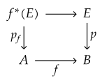
is flat over $H$. Given $g:T\to H$, pull back the diagram:

$$\mathcal Z_T = \mathcal Z\times_H T \hookrightarrow X\times_S T.$$

This is the family classified by $g$. Conversely, any family in the Hilbert functor determines one and only one $g$.

The universal object is not usually one fiber containing the others. It is a family whose base is the parameter scheme. Its total space can be as complicated as the objects vary.

If $T$ has nilpotents, the map $T\to H$ can encode an infinitesimal deformation. Thus the scheme structure of $H$, not just its closed points, matters. Tangent directions at $[Z]$ correspond in standard settings to homomorphisms

$$\operatorname{Hom}_{\mathcal O_Z}(\mathcal I_Z/\mathcal I_Z^2,\mathcal O_Z),$$

or equivalently suitable $\operatorname{Hom}(\mathcal I_Z,\mathcal O_Z)$ formulations. Obstructions can prevent tangent directions from extending to actual curves in $H$.

This modern tangent description faithfully explains what nonreduced structure can record. It should not be attributed sentence-for-sentence to the 1961 exposé. The historical theorem guarantees a scheme on which later deformation theory can operate.

The universal family also controls base change. If $S'\to S$, the Hilbert scheme of the base-changed projective scheme relates by base change under the theorem’s hypotheses:

$$\operatorname{Hilb}^{P}_{X/S}\times_S S' \cong \operatorname{Hilb}^{P}_{X_{S'}/S'}.$$

This is representability’s reward: compatibility follows from the functor’s definition and uniqueness, once hypotheses align.

Points moving and points colliding

The Hilbert scheme of $d$ points on a space provides an intuitive case. A reduced length-$d$ subscheme over an algebraically closed field looks like $d$ distinct points. As points collide, the flat limit is often nonreduced. The Hilbert scheme includes that limit.3434Grothendieck, “Techniques de construction et théorèmes d’existence en géométrie algébrique. IV. Les schémas de Hilbert”; The Stacks Project Authors, The Stacks Project.

For the affine or projective line, length-$d$ subschemes have especially tractable parameter spaces. A monic polynomial of degree $d$ defines a finite flat subscheme, and repeated roots produce nonreduced fibers. The coefficients parameterize both separated and collided configurations.

In dimension at least two, punctual Hilbert schemes become richer. Multiple nonisomorphic nonreduced structures can sit at one support point. The parameter space records directions and higher-order structures that the symmetric product of point sets forgets.

The difference between the Hilbert scheme and a symmetric product is a precise version of the chapter’s theme. A set of unordered points is not enough for a family closed under collision. Scheme structure on the members and parameter space retains the limiting information.

This example explains why representability and schemes are inseparable. If Grothendieck had required every member to be a reduced variety, the family functor would not be stable under natural specialization.

From Hilbert space to moduli space

The Hilbert scheme parameterizes embedded subschemes $Z\subseteq\mathbb P^n$ or $X$. A moduli problem for abstract varieties usually wants to forget the embedding. Different points of the Hilbert scheme can represent isomorphic abstract objects embedded in different coordinates.3535Grothendieck, “Techniques de construction et théorèmes d’existence en géométrie algébrique. IV. Les schémas de Hilbert”; The Stacks Project Authors, The Stacks Project.

The projective linear group acts by changing coordinates. One might try to form a quotient. Stabilizer groups record automorphisms of the embedded object. Orbits may fail to be closed, and naive orbit spaces may not be schemes with the desired universal property.

This is the terrain on which geometric invariant theory would develop, especially through David Mumford’s work in the 1960s. Grothendieck’s quotient and Hilbert exposés supplied central foundations and explicitly identified the quotient obstacle. Mumford’s GIT has its own authorship and should not be treated as an automatic corollary of FGA.

The sequence—embed, parameterize by Hilbert, restrict to a suitable locus, quotient by projective transformations—became a standard moduli strategy. Each arrow carries a theorem. Boundedness chooses embeddings; Hilbert representability supplies a projective scheme; stability conditions improve orbits; quotient theory constructs a moduli space.

Fine moduli may still fail because automorphisms prevent a universal family. A coarse moduli space may exist. A stack may retain the full groupoid. The Hilbert scheme solves the embedded representability problem, not every classification problem downstream.

The sheaf test

A representable functor must satisfy descent. If maps $T_i\to T$ cover $T$, morphisms $T\to M$ are determined by compatible morphisms $T_i\to M$. Therefore $h_M$ is a sheaf for topologies in which schemes descend, including the fpqc topology.3636Grothendieck and Dieudonné, “Éléments de géométrie algébrique III: Étude cohomologique des faisceaux cohérents, première partie”; Grothendieck, “Technique de descente et théorèmes d’existence en géométrie algébrique. II. Le théorème d’existence en théorie formelle des modules”.

This gives a necessary condition. A raw moduli presheaf that fails the sheaf condition cannot be represented by a scheme. One may sheafify it, but sheafification can alter the naive set of objects and equivalences.

Line bundles illustrate the issue. Isomorphism classes of line bundles form a group, but relative Picard functors often quotient by line bundles pulled back from the test base and require fppf or étale sheafification. Without the correct sheaf, gluing families can fail.

The condition also links representability to Grothendieck topologies. Covers need not be only open subsets; faithfully flat morphisms can detect and glue. The site and topos formalism of the next Part will make this systematic.

One should not claim that the full later hierarchy of topologies was already formalized in exposé 195. The chronological point is narrower: Grothendieck’s representability program and faithfully flat descent were already inseparable by 1959–1961.

Hom and Isom functors

Given $S$-schemes $X$ and $Y$, define

$$\underline{\operatorname{Hom}}_S(X,Y)(T) = \operatorname{Hom}_T(X_T,Y_T).$$

If represented, the resulting $S$-scheme parameterizes maps from $X$ to $Y$ in families. An open or locally closed subfunctor may parameterize isomorphisms. Taking $X=Y$ can produce an automorphism group scheme.

Grothendieck’s October 1959 letter explores such relative Hom constructions and their reduction to section functors. It notes cases of existence and counterexamples.3737Grothendieck and Serre, Correspondance Grothendieck–Serre, 101–6.

The example shows representability applying not only to objects but to arrows. A category of schemes can itself possess schemes of morphisms under suitable properness and projectivity hypotheses.

Automorphism schemes then make stabilizers geometric. A family may have finite, positive-dimensional, reduced, or infinitesimal automorphisms. The last type is invisible if one records only automorphism groups of geometric points as abstract sets.

This precision sharpens the moduli obstruction in the November 5 letter. An automorphism problem has more structure than the informal phrase “too much symmetry” conveys. A nontrivial group scheme acts, and its variation affects descent and quotient representability.

Existence of Hom schemes is not unrestricted. Properness of the source, quasi-projectivity of the target, finiteness conditions, and chosen categories matter. The notation $\underline{\operatorname{Hom}}$ may denote a functor even when no representing scheme exists.

Weil restriction as representability

For $T\to S$ and a $T$-scheme $X$, restriction of scalars seeks an $S$-scheme $\operatorname{Res}_{T/S}X$ satisfying

$$\operatorname{Hom}_S(S',\operatorname{Res}_{T/S}X) \cong \operatorname{Hom}_T(T\times_S S',X).$$

This is another representability problem. Over finite field extensions it recasts a variety defined over the larger field as an object over the smaller field of greater dimension.

Weil used such ideas; Grothendieck’s correspondence calls the construction a Weil operation and explores its relation to Greenberg-type functors and relative Hom. The letters also acknowledge existence limits.3838Grothendieck and Serre, Correspondance Grothendieck–Serre, 101–7.

The attribution is layered. André Weil’s name properly attaches to restriction of scalars and earlier descent. Grothendieck placed the operation in the general functor-of-points setting and investigated representability for schemes.

The construction reinforces a central lesson: many geometric objects are best defined by what maps into them must mean. The formula is the definition; equations or charts are the existence proof.

Local representability is not global representability

A deformation functor may be pro-representable near one object. This gives a formal local parameter ring. It does not provide a global moduli scheme containing all objects.3939Grothendieck, “Technique de descente et théorèmes d’existence en géométrie algébrique. II. Le théorème d’existence en théorie formelle des modules”; Grothendieck and Dieudonné, “Éléments de géométrie algébrique III: Étude cohomologique des faisceaux cohérents, première partie”.

Several gaps remain. Local rings must be algebraized to neighborhoods. Neighborhoods must be glued. The functor must be bounded enough to fit in a set or finite-type union. Automorphisms must be controlled. Components can have different dimensions.

Grothendieck’s strategy combined local formal methods with global projective parameter spaces. The Hilbert scheme succeeds because embeddings and a fixed polynomial give boundedness, while the Grassmannian gives a global projective container.

The comparison explains why a general existence theorem was so ambitious. It sought criteria spanning infinitesimal deformation, formal effectivity, descent, and global construction.

Later representability theorems separated these requirements more systematically. Historical accuracy requires saying “the program sought” when the 1959 letter projects, “the exposé proved” when FGA states a theorem, and “later theory established” for subsequent criteria.

Natural transformations as constructions

Once two functors are represented, a natural operation between the classified families becomes a morphism between representing schemes. This is Yoneda used constructively.4040Grothendieck and Dieudonné, “Éléments de géométrie algébrique III: Étude cohomologique des faisceaux cohérents, première partie”; Grothendieck, “Technique de descente et théorèmes d’existence en géométrie algébrique. II. Le théorème d’existence en théorie formelle des modules”.

For example, taking the support cycle of a subscheme may define a map from a suitable Hilbert scheme to a Chow space under hypotheses. Tensoring line bundles defines a group law on a Picard functor and, when represented, a group-scheme law. Composing maps defines morphisms among Hom schemes.

Associativity and identity can be checked at the functor level. Yoneda then transfers them to the representing object. A group scheme is a scheme $G$ for which $G(T)$ is naturally a group for every $T$, with the operations represented by morphisms

$$G\times_S G\to G,\qquad G\to G,\qquad S\to G.$$

This practice helps explain why category theory was not an external philosophy in EGA. It converted operations on families into geometry and coherence into diagrams.

There is a subtle limit. Not every pointwise operation is natural, and not every natural functor is representable. Functorial thinking supplies a test and a translation, not automatic geometry.

The status of universality

The word “universal” can inflate a narrative. The universal family on a Hilbert scheme is universal relative to a specified functor: closed subschemes of a fixed projective $X$, flat over the test base, with fixed Hilbert polynomial. Change the equivalence, ambient scheme, or allowed families and the universal property changes.4141Grothendieck, “Technique de descente et théorèmes d’existence en géométrie algébrique. II. Le théorème d’existence en théorie formelle des modules”; Grothendieck and Dieudonné, “Éléments de géométrie algébrique III: Étude cohomologique des faisceaux cohérents, première partie”.

Similarly, a universal deformation may be only versal when uniqueness fails. A coarse moduli space has a different universal property from a fine one. An initial or final object is universal in a category but need not classify a moduli problem.

Grothendieck’s program taught mathematicians to seek universal properties; it also made precise qualifiers unavoidable. The grandeur of a construction lies in the exact range over which it is universal, not in omission of the range.

This precision protects attribution. Yoneda’s universal correspondence is categorical. Hilbert’s polynomial is numerical. Grothendieck’s Hilbert scheme is a relative representing object. The words overlap, but the contributions do not.

Universal problems before the functorial turn

Universal constructions long predated 1960. Free groups, tensor products, algebraic closures under qualified uniqueness, Jacobians, and parameter spaces were characterized by mapping properties or canonical correspondences. Hilbert and Poincaré asked for universal families in their own languages. Category theory did not invent the mathematical desire for a best or most general object.4242Grothendieck, “Technique de descente et théorèmes d’existence en géométrie algébrique. II. Le théorème d’existence en théorie formelle des modules”; Grothendieck and Dieudonné, “Éléments de géométrie algébrique III: Étude cohomologique des faisceaux cohérents, première partie”.

What changed was systematic formulation. A universal problem became representability of a functor. Uniqueness followed from Yoneda. Base change was built into naturality. Algebraic structures on the solution could be transferred from operations on the functor.

This reformulation separates three tasks. First, define the functor correctly on all test objects. Second, prove that a representing object exists. Third, study the geometry of that object. Earlier parameter methods often combined the tasks through coordinates.

The new separation did not make coordinate constructions obsolete. The Hilbert scheme proof uses homogeneous coordinates and Grassmannians to solve the second task. Once constructed, however, the object is identified by a coordinate-free universal property.

The history should therefore avoid a false opposition between classical concrete geometry and categorical abstraction. Representability turns concrete construction into a universal result. It needs both.

The Picard functor more carefully

For a proper flat morphism $f:X\to S$, a first attempt might define

$$T\longmapsto\operatorname{Pic}(X_T),$$

the group of isomorphism classes of line bundles on $X_T$. But a line bundle pulled back from $T$ becomes trivial on each fiber and should not change the relative class. One therefore considers a quotient by $\operatorname{Pic}(T)$ in a standard formulation and then addresses sheafification in an appropriate topology.

Even this sentence hides hypotheses. A section of $X\to S$ can rigidify line bundles. Cohomological flatness can affect representability. The identity component, separatedness, and finite type require conditions. Picard schemes may be nonreduced in positive characteristic.

The complexity explains why the Hilbert scheme is an auxiliary rather than the final answer. Effective divisors can be parameterized as subschemes. Their line bundles map to Picard classes. Taking a quotient by linear equivalence or using descent should produce the Picard object where theorems apply.

Exposé 212 in February 1961 describes Picard as a quotient of schemes of positive divisors or projective embeddings. Exposé 221 in May says the next lecture will combine quotient and Hilbert techniques to construct Picard schemes under general conditions.4343Grothendieck, “Techniques de construction et théorèmes d’existence en géométrie algébrique. III. Préschémas quotients,” 99; Grothendieck, “Techniques de construction et théorèmes d’existence en géométrie algébrique. IV. Les schémas de Hilbert,” 249.

The February and May 1962 Picard exposés delivered the next stage. Ending this chapter in 1961 leaves the functor at a productive threshold. This is not artificial truncation; it preserves the Part’s chronology and prevents announcement from becoming achievement.4444Grothendieck, “Technique de descente et théorèmes d’existence en géométrie algébrique. V. Les schémas de Picard: Théorèmes d’existence”; Grothendieck, “Technique de descente et théorèmes d’existence en géométrie algébrique. VI. Les schémas de Picard: Propriétés générales”.

The Picard example also displays cumulative credit. Divisor classes, Jacobians, and Picard varieties were classical achievements developed by many mathematicians. Grothendieck’s relative Picard scheme generalized and represented the family functor. The new theorem does not absorb the old theories’ authorship.

Divisors and representability

An effective Cartier divisor on $X_T$ is locally defined by one non-zero-divisor and corresponds to an invertible ideal sheaf under suitable conditions. Such divisors can form a functor in $T$.4545Grothendieck, “Techniques de construction et théorèmes d’existence en géométrie algébrique. III. Préschémas quotients”; Grothendieck, “Techniques de construction et théorèmes d’existence en géométrie algébrique. IV. Les schémas de Hilbert”; The Stacks Project Authors, The Stacks Project.

When $X\to S$ is projective, divisors with fixed Hilbert polynomial are points of a Hilbert scheme. The universal subscheme restricts to a universal divisor on an open locus where the Cartier condition holds.

This is a typical representability pattern: start with a large Hilbert functor, identify the property defining the desired objects, prove that property cuts out an open or locally closed subfunctor, and inherit representation.

The construction translates a local condition—one equation that is not a zero divisor—into a geometric locus in a parameter space. It demonstrates why studying morphism properties in EGA II was prerequisite to moduli.

Not every divisor problem is represented by a projective scheme, and not every cycle is Cartier. Weil divisors on normal schemes, Cartier divisors, and closed subschemes carry different information. Representability requires the correct functor, not a generic word “divisor.”

Necessary conditions do not suffice

A representable functor on schemes preserves certain limits. Since maps into $M$ turn colimits in test schemes into limits of sets where those colimits exist, $F$ must have matching compatibility. It must also be an fpqc sheaf. Its diagonal, viewed as an Isom functor, must have appropriate representability properties for geometric applications.4646Grothendieck and Dieudonné, “Éléments de géométrie algébrique III: Étude cohomologique des faisceaux cohérents, première partie”; Grothendieck, “Technique de descente et théorèmes d’existence en géométrie algébrique. II. Le théorème d’existence en théorie formelle des modules”.

These necessary conditions guide tests. If a functor fails descent or treats an inverse limit incompatibly, it cannot be represented by a scheme.

But satisfying obvious conditions need not provide a finite-type scheme. The functor may be an infinite disjoint union, an algebraic space, a formal scheme, a stack, or something less geometric. Boundedness and algebraization remain.

The projected general existence theorem therefore required more than Yoneda. It had to join local deformation, formal effectivity, descent, and global boundedness.

The October 1959 letter should be read as a research agenda toward such criteria. The February 1960 exposé establishes important components. The May 1961 Hilbert theorem verifies them for one fundamental class. No single 1959–1961 theorem represents every reasonable functor.

A failure caused by automorphisms

Take a moduli problem in which an object $E$ has a nontrivial automorphism $g$. Cover a base $T$ by $T_i$. On overlaps, local families can be glued by transition isomorphisms. Changing those isomorphisms by automorphisms may alter the global family without altering local isomorphism classes.

If the functor records only the set of local isomorphism classes, it cannot see the cocycle. The sheaf condition can fail: compatible-looking classes do not determine a unique global class.

Rigidification adds data so that automorphisms become trivial or controlled. For a curve, marked points or level structures can help. For a vector bundle, a framing along a divisor or at points can help. The classifying map then has a chance to be unique.

Stacks take the other route. Instead of discarding isomorphisms, they make the groupoid of families the value over $T$. Descent is then stated for objects and arrows. The automorphism group becomes a stabilizer rather than an obstruction hidden by quotienting.

Grothendieck’s November 5 letter identifies automorphisms as preventing descent and suggests added structures. The letter contains the problem and one strategy. It does not contain the mature definition or representability theory of algebraic stacks.4747Grothendieck and Serre, Correspondance Grothendieck–Serre, 107–10.

This boundary is especially important in biography because later theory can make an early remark look omniscient. The accurate claim is more valuable: he saw, while building representability criteria, that symmetry was an obstruction rooted in descent.

The geometry of the representing scheme

Once a functor is represented, attention shifts to whether the scheme is of finite type, proper, smooth, separated, or reduced, to its components, and to the meaning of its tangent and obstruction spaces.4848Grothendieck, “Technique de descente et théorèmes d’existence en géométrie algébrique. II. Le théorème d’existence en théorie formelle des modules”; Grothendieck and Dieudonné, “Éléments de géométrie algébrique III: Étude cohomologique des faisceaux cohérents, première partie”.

For a Hilbert scheme, a point $[Z]$ can be smooth even when $Z$ is singular, or singular even when $Z$ is smooth, depending on embedded deformation theory. Components can meet. Expected dimension can fail.

Thus representability is a beginning, not a classification completed. It creates an object to which geometry can be applied.

The universal family transfers information in both directions. Geometry of $H$ describes how subschemes deform; special subschemes can create singularities in $H$. Universal maps produce loci with specified properties.

This recursive quality is central to Grothendieck’s method. Geometry builds a space of geometries, then studies that space by the same scheme-theoretic tools. The moduli object is not external metadata.

The recursion also creates scale. Parameter spaces require their own compactifications, stratifications, and cohomology. A foundational method generates new objects faster than one treatise can exhaust them.

Dieudonné and the categorical preliminaries

Exposé 195 is authored by Grothendieck. EGA III’s representable-functor section belongs to the treatise written in collaboration with Dieudonné. The distinction between lecture and systematic reference again matters.4949Grothendieck and Dieudonné, “Éléments de géométrie algébrique I: Le langage des schémas”; Grothendieck and Dieudonné, “Éléments de géométrie algébrique III: Étude cohomologique des faisceaux cohérents, première partie”; Grothendieck, “Technique de descente et théorèmes d’existence en géométrie algébrique. II. Le théorème d’existence en théorie formelle des modules”; Grothendieck and Serre, Correspondance Grothendieck–Serre.

Grothendieck’s lecture moves rapidly from category $\mathcal C$ and $h_X$ to pro-representability and formal existence. EGA Chapter 0 expands definitions, proves the Yoneda bijection, develops full subcategories and fully faithful functors, and places projective limits in the framework.

This expansion is characteristic of Dieudonné’s redactional contribution. The printed evidence does not permit assignment of each proposition, but the collaboration formula and correspondence support his role in turning current ideas into ordered preliminaries.

Serre’s correspondence supplies another layer. His October question about categories and the multiplodocus elicited Grothendieck’s report. His later editorial notes explain which projected chapters never appeared and which statements changed. Representability’s history is visible because one interlocutor preserved both mathematical content and correction.

Yoneda remains the origin of the lemma. Bourbaki and category theorists supplied a language in circulation. EGA made that language unavoidable for a generation of algebraic geometers. These are different contributions, and the chapter needs all of them.

Five dated documents

The representability program’s growth can be fixed to five documents. First, the October 31, 1959 letter joins descent, formal existence, and functors of points. Second, the November 5 letter diagnoses automorphisms in moduli descent.5050Grothendieck and Dieudonné, “Éléments de géométrie algébrique III: Étude cohomologique des faisceaux cohérents, première partie”; Grothendieck, “Technique de descente et théorèmes d’existence en géométrie algébrique. II. Le théorème d’existence en théorie formelle des modules”; Grothendieck, “Techniques de construction et théorèmes d’existence en géométrie algébrique. III. Préschémas quotients”; Grothendieck, “Techniques de construction et théorèmes d’existence en géométrie algébrique. IV. Les schémas de Hilbert”; Grothendieck and Serre, Correspondance Grothendieck–Serre.

Third, exposé 195 in February 1960 opens with representable and pro-representable functors and develops formal existence. Fourth, exposé 212 in February 1961 treats quotient preschemes and states open problems. Fifth, exposé 221 in May 1961 constructs Hilbert schemes under projective hypotheses.

EGA III.1, also in 1961, installs representable functors in the treatise’s preliminaries. It can be considered a sixth document of consolidation rather than a separate step in discovery.

The dates prevent compression into one “representability theorem.” There was a method, several theorems, unsolved quotients, and a moving publication program.

The sequence also shows that FGA and EGA had distinct rhythms. Bourbaki exposés could announce recent work and open questions. EGA supplied foundational detail. Neither alone represents the period.

The reach and boundary of 1961

By the end of 1961, the Hilbert functor gave a decisive success. Relative Hom and Weil restriction had important cases and ongoing questions. Quotients were partially constructed and partially open. Picard schemes were imminent but not yet delivered in the dated exposés. General moduli with automorphisms remained beyond schemes.5151Grothendieck and Dieudonné, “Éléments de géométrie algébrique III: Étude cohomologique des faisceaux cohérents, première partie”; Grothendieck, “Technique de descente et théorèmes d’existence en géométrie algébrique. II. Le théorème d’existence en théorie formelle des modules”; Grothendieck, “Techniques de construction et théorèmes d’existence en géométrie algébrique. III. Préschémas quotients”; Grothendieck, “Techniques de construction et théorèmes d’existence en géométrie algébrique. IV. Les schémas de Hilbert”; Grothendieck and Serre, Correspondance Grothendieck–Serre; Grothendieck, “Technique de descente et théorèmes d’existence en géométrie algébrique. V. Les schémas de Picard: Théorèmes d’existence”; Grothendieck, “Technique de descente et théorèmes d’existence en géométrie algébrique. VI. Les schémas de Picard: Propriétés générales”.

This mixed ledger is historically healthier than a single verdict. Representability had become a central way to formulate existence. It had not become a universal existence machine.

Its influence can already be seen in vocabulary. One asks whether a functor is representable, rather than only whether a space “of” objects exists. One searches for a universal family. One tests base change and descent. One treats failure as structural.

The next decades would extend the answer through algebraic spaces, stacks, and broader criteria. Those developments confirm the fertility of the question while demonstrating the insufficiency of the 1961 category for every problem.

Why closed points are not a moduli theorem

Suppose a variety $M$ has closed points in bijection with isomorphism classes of objects over an algebraically closed field. The bijection is evidence of parameterization, but not representability.5252Grothendieck and Dieudonné, “Éléments de géométrie algébrique III: Étude cohomologique des faisceaux cohérents, première partie”; Grothendieck, “Technique de descente et théorèmes d’existence en géométrie algébrique. II. Le théorème d’existence en théorie formelle des modules”.

First, it says nothing about families over a positive-dimensional base. A map $T\to M$ may fail to produce the intended family, or several nonisomorphic families may induce the same map on closed points.

Second, it says nothing about fields that are not algebraically closed. Rational points can encode descent forms, and residue fields matter.

Third, it says nothing about infinitesimal families. Maps from dual numbers detect tangent directions and nonreduced structure on $M$. A reduced point set cannot carry obstruction theory.

Fourth, it says nothing about universality. Even if a family is assigned to every point, there may be no one family on $M$ whose pullbacks produce all others.

Fifth, it says nothing about automorphisms. A universal family may fail because local families glue only up to nonunique isomorphism.

The Hilbert scheme succeeds because the theorem answers every objection in a specified embedded setting. It represents a functor on all $S$-schemes, carries a universal closed subscheme, and includes infinitesimal bases. Its closed points are only one visible layer.

This distinction changed how algebraic geometers evaluated construction. A parameter count or coordinate variety could be useful without being a fine moduli space. The universal property became the acceptance test.

The test can be too strong for the desired application. A coarse moduli space may suffice for invariants even without a universal family. Representability is not the only legitimate form of classification.

Grothendieck’s method supplies vocabulary for choosing: fine, coarse, formal, pro-representable, algebraic space, or stack in later language. Each word states what the constructed object promises.

The philosophical force lies in that exact promise. Existence is not certified by resemblance between points and answers. It is certified by natural behavior under every allowed change of base.

This standard also protects history. Earlier Chow varieties and parameter spaces should not be dismissed for failing a later functorial definition they were not built to satisfy. Grothendieck’s Hilbert theorem should not be reduced to another point-bijection construction. The works answer related questions at different levels.

By insisting on families, representability converts classification from a catalog into geometry. The catalog’s pages can themselves bend, thicken, specialize, and descend.

The discipline of the universal element

A proposed moduli space can be tested through its universal element $\xi\in F(M)$: its fibers, its pullback along infinitesimal maps, whether every family arises from it, and whether the classifying map is unique.5353Grothendieck, “Technique de descente et théorèmes d’existence en géométrie algébrique. II. Le théorème d’existence en théorie formelle des modules”; Grothendieck and Dieudonné, “Éléments de géométrie algébrique III: Étude cohomologique des faisceaux cohérents, première partie”.

These questions expose weak constructions quickly. A coordinate quotient may label orbits but lack a universal family. A set of invariants may identify generic objects but collapse special ones. A formal local ring may classify infinitesimal deformations but not algebraic families globally.

The universal element also makes proofs economical. To define an operation on all families, define it on $\xi$ and prove compatibility with pullback. To compare two representations, use the classifying maps of their universal elements; Yoneda makes them inverse.

For the Hilbert scheme, $\xi$ is the universal closed subscheme. For a Grassmannian, it is the universal quotient bundle. For a Picard scheme under suitable conditions, it is subtler because a universal line bundle may require rigidification or exist only up to pullback.

The examples show why “fine moduli” is a strong claim. It asserts not only points and geometry but a universal object with exact naturality.

Grothendieck’s representability method disciplined ambition by making this claim checkable. It also made partial successes nameable: coarse space, formal hull, algebraic space, or stack in later vocabulary.

The historical achievement is a standard of evidence for existence. A space is not accepted because its name matches the objects. It must perform the universal relationship.

Credit for representability

Representability concentrates several lineages. Yoneda receives credit for the categorical result that identifies natural transformations from a representable functor. Hilbert receives credit for the polynomial and foundational algebra behind bounded projective families; Grassmann and Chow name earlier parameter traditions. Weil and Cartier enter through descent. Serre enters through prior geometry, criticism, and the correspondence that documents the program. Grothendieck receives credit for making representability a central geometric method and for constructing the Hilbert scheme in the relative scheme setting. Dieudonné receives credit for collaboration in EGA’s systematic categorical exposition. Picard existence remains dated to the later exposés, and stack solutions remain attached to their subsequent authors. The allocation matters because a universal property can absorb old results so smoothly that their origins disappear. This checkpoint keeps invention, synthesis, proof, redaction, and later extension from becoming one undifferentiated achievement. The distinction is especially important for moduli, where a pointwise parameter set, a fine representing scheme, a coarse space, and a stack answer different questions. Later vocabulary clarifies these differences, but it must not be inserted into 1961 as though all solutions already existed there then in mature form.5454Grothendieck and Dieudonné, “Éléments de géométrie algébrique I: Le langage des schémas”; Grothendieck and Dieudonné, “Éléments de géométrie algébrique III: Étude cohomologique des faisceaux cohérents, première partie”; Grothendieck, “Technique de descente et théorèmes d’existence en géométrie algébrique. I. Généralités. Descente par morphismes fidèlement plats”; Grothendieck, “Technique de descente et théorèmes d’existence en géométrie algébrique. II. Le théorème d’existence en théorie formelle des modules”; Grothendieck, “Techniques de construction et théorèmes d’existence en géométrie algébrique. IV. Les schémas de Hilbert”; Grothendieck and Serre, Correspondance Grothendieck–Serre; Serre, “Faisceaux algébriques cohérents”; Yoneda, “On the Homology Theory of Modules”; Grothendieck, “Technique de descente et théorèmes d’existence en géométrie algébrique. V. Les schémas de Picard: Théorèmes d’existence”; Grothendieck, “Technique de descente et théorèmes d’existence en géométrie algébrique. VI. Les schémas de Picard: Propriétés générales”.

Representability also changes the burden of proof in biography. A later space with the expected name cannot be credited backward to an early program without the construction and universal property. The dated record must show what functor was defined, what hypotheses were imposed, and what object was proved to represent it. This rule preserves Grothendieck’s 1961 Hilbert theorem and preserves later authorship for the solutions still missing. Universal language makes this historical test clear, exact, and strict.

The same rule keeps stack language explanatory rather than proprietary: it clarifies the obstruction without turning the 1959 letter into the later theory.

Existence as relationship

Grothendieck’s method relocates existence. A parameter space exists adequately when it occupies the correct relationship to every test scheme. This is stronger than exhibiting a set and subtler than writing equations in one chart.5555Grothendieck and Dieudonné, “Éléments de géométrie algébrique III: Étude cohomologique des faisceaux cohérents, première partie”; Grothendieck, “Technique de descente et théorèmes d’existence en géométrie algébrique. II. Le théorème d’existence en théorie formelle des modules”.

The philosophical temptation is to say that an object is its relations. Yoneda supports a precise categorical statement: an object is determined up to isomorphism by its representable functor and natural transformations. It does not say objects have no internal structure or that all nonmathematical identity is relational.

Within geometry, the statement has radical practical force. Coordinate choices become secondary to universal properties. Base change becomes built into classification. A universal family, not a bijection of closed points, certifies the parameter space.

The method is also collective. Yoneda supplied the categorical lemma. Hilbert, Grassmann, Chow, and others supplied classical structures. Weil and Cartier supplied descent settings. Serre’s questions and earlier geometry shaped problems. Dieudonné helped turn the language into EGA. Grothendieck assembled these resources into a construction program and proved the Hilbert representability theorem.

By May 1961 one major question had answered itself geometrically: families of projective subschemes with fixed Hilbert polynomial were represented by a projective scheme carrying a universal family. The success made representability a standard ambition. The failures around quotients and automorphisms ensured it would not become a mechanical one.

The method required places for teaching, criticism, writing, and publication. IHÉS still worked from borrowed Paris rooms, but its appointments, visitors, and journal already connected a developing research community.