A Machine for Weil

A formula in the Bourbaki record

Grothendieck’s Bourbaki exposé 279 bears the title Formule de Lefschetz et rationalité des fonctions L. It belongs to the 1964–65 seminar session and was printed in 1966, on pages 41 through 55 of the collected volume. That double date is the proper doorway into the machine. By the session in which the program was explained, one part of Weil’s conjectural package—rationality—had already been proved by Bernard Dwork. The claim was no longer that only a new cohomology could establish the fact. It was that cohomology could explain why the fact belonged to a larger geometry.11Alexandre Grothendieck, “Formule de Lefschetz et rationalité des fonctions L,” Exposé 279, Séminaire Bourbaki, vol. 9 (1964–1966), 1966, 41–55, https://www.numdam.org/item/SB_1964-1966__9__41_0/.

The exposé’s two nouns, Lefschetz formula and L-functions, joined topological method to arithmetic output. A Lefschetz fixed-point formula relates fixed points of a map to traces of the induced action on cohomology. Over a finite field, the relevant map is Frobenius. Its fixed points over extension fields are precisely the rational points being counted. If a suitable cohomology theory existed, repeated point counts could become traces of powers of one operator.

This was the sense in which Grothendieck sought a machine. The input would be a scheme or variety over a finite field, together with a sheaf when an L-function required coefficients. The internal mechanism would be étale and ℓ-adic cohomology, direct and inverse images, compact supports, duality, and Frobenius. The output would be a determinant expression whose algebraic shape forced rationality and organized the functional equation.

No physical machine operates by analogy, and neither did this one. Each gear was a theorem. Cohomology groups had to be finite-dimensional. Frobenius had to act. Traces had to equal fixed-point counts. Compact support had to behave functorially. Duality had to produce the reciprocal relation behind a functional equation. Change of base had to connect fibers. A missing compatibility could stop the calculation.

The program’s magnitude becomes clearer by returning to the problem before the machine existed.

Weil’s finite-field horizon

For a variety $X$ over the finite field $\mathbf F_q$, let $$N_n=\#X(\mathbf F_{q^n}).$$ The zeta function packages every extension-field count: $$Z(X,t)=\exp\left(\sum_{n\ge1}N_n\frac{t^n}{n}\right).$$ The exponential is initially a formal power series. Rationality says that this apparently infinite record is the expansion of a rational function.22André Weil, “Numbers of Solutions of Equations in Finite Fields,” Bulletin of the American Mathematical Society 55, no. 5 (1949): 497–508, https://doi.org/10.1090/S0002-9904-1949-09219-4.

André Weil’s 1949 paper predicted much more for nonsingular projective varieties. The zeta function should be rational; it should satisfy a functional equation; its factorization should have degrees governed by topological Betti numbers; and the reciprocal roots should have absolute values prescribed by their cohomological degree, an analogue of the Riemann hypothesis. Historical summaries divide and order the assertions differently, so the fourfold list should be read as a modern guide to the package, not as a replacement for Weil’s wording.33Weil, “Numbers of Solutions of Equations in Finite Fields”.

For the projective line the count is elementary: $\#\mathbf P^1(\mathbf F_{q^n})=q^n+1$, giving $$Z(\mathbf P^1,t)=\frac{1}{(1-t)(1-qt)}.$$ The two denominator factors resemble contributions from cohomological degrees zero and two. For a smooth projective curve of genus $g$, the numerator should have degree $2g$, echoing the first Betti number of the corresponding complex Riemann surface. The analogy suggested that cohomology was not decoration applied to the answer; it was the hidden finite-dimensional source of the factors.

The finite field supplies a canonical endomorphism. Arithmetic Frobenius raises coordinates to the $q$-th power; geometric Frobenius is its inverse under a common convention. Authors differ about which one acts in a displayed formula. The convention changes eigenvalues by inversion and must be fixed. What matters for the program is that $X(\mathbf F_{q^n})$ can be recognized as fixed points of an appropriate $n$-th power of Frobenius after passing to an algebraic closure.

Classical topology offered the model. If a continuous map on a suitable compact space has isolated fixed points, the Lefschetz number—the alternating sum of traces on cohomology—can count them with multiplicities. Weil’s insight was that his conjectures had the formal appearance of such a theory. But a variety in characteristic $p$ did not come with singular cohomology over the rational numbers. The missing theory had to be algebraic enough to exist over finite fields and topological enough to satisfy trace and duality.

Grothendieck’s 1958 ICM address made that cohomological program explicit. The scheme language then widened the domain on which it could be pursued. SGA 1 supplied finite étale covers and the fundamental group. SGA 4 built the étale topos and its cohomology. By the middle of the 1960s, the pieces could be directed toward Frobenius.44Grothendieck, “The Cohomology Theory of Abstract Algebraic Varieties”.

Dwork before the machine

In 1960 Bernard Dwork proved the rationality of the zeta function of an algebraic variety using p-adic analysis. This fact sets a firm boundary on any triumphalist account. Grothendieck and his collaborators did not first establish rationality by inventing étale cohomology. The theorem existed before SGA 4’s seminar year and before SGA 5.55Dwork, “On the Rationality of the Zeta Function of an Algebraic Variety”.

Dwork’s proof also sharpened the philosophical difference between proving a fact and placing it in an architecture. A p-adic analytic argument could force the generating series to be rational. It did not by itself supply the Betti-number interpretation, Poincaré duality, or a general geometric theory of Frobenius eigenvalues. The cohomological route promised to make rationality one shadow of a finite-dimensional object and to link it to the other conjectures.

The distinction should not be turned into a hierarchy in which “explanation” erases proof. Dwork solved the problem he addressed. Grothendieck’s program changed the question by asking for a system that produced the answer and survived broader operations. Both are mathematical achievements of different kinds. The history is more accurate when their methods remain distinct.

There was also a productive pressure in the prior proof. Once rationality no longer served as the sole test, the cohomological theory had to justify its size through coherence and reach. It should explain L-functions with sheaf coefficients as well as the zeta function of one smooth projective variety. It should work in families, handle nonproper schemes through compact supports, and support duality. The target expanded.

Grothendieck’s Bourbaki title in 1964–65 therefore did not announce a race already won by another method. It joined rationality to a Lefschetz formula because the formula identified the sought mechanism. The point was to derive the rational function as an alternating product of characteristic polynomials, making its factors geometric.

From finite coefficients to ℓ-adic spaces

Étale cohomology behaved well first with finite coefficients whose order was invertible on the scheme. Over characteristic $p$, choose a prime $\ell\ne p$ and consider $$H^i_{\acute et}(X_{\overline{\mathbf F}_q}, \mathbf Z/\ell^n\mathbf Z).$$ These groups carry Frobenius action and, under suitable finiteness hypotheses, are finite.

One finite coefficient ring is not enough for characteristic-zero linear algebra. The compatible tower over all $n$ leads toward the ℓ-adic integers: $$H^i(X,\mathbf Z_\ell)\ \sim\ \underset{\longleftarrow}{\lim}_n H^i(X,\mathbf Z/\ell^n\mathbf Z),$$ with technical care about inverse limits, and then $$H^i(X,\mathbf Q_\ell)=H^i(X,\mathbf Z_\ell)\otimes_{\mathbf Z_\ell}\mathbf Q_\ell.$$ The tilde in the first display is a warning: historical and modern definitions require hypotheses and derived-limit control; one must not assume that ordinary sheaf cohomology commutes with every inverse limit.66Illusie, Cohomologie ℓ-adique et fonctions L (SGA 5); Milne, Étale Cohomology.

The auxiliary prime $\ell$ differs from the field characteristic. It creates a characteristic-zero coefficient field $\mathbf Q_\ell$, where Frobenius can be studied by linear algebra. The eigenvalues are algebraic numbers viewed through embeddings into ℓ-adic fields, while the Riemann-hypothesis assertion concerns their complex absolute values. The machine would have to bridge these worlds without making the answer depend on $\ell$.

This construction is sometimes described as replacing missing rational cohomology. The phrase is useful if it does not suggest that $\mathbf Q_\ell$ is literally $\mathbf Q$ or that the resulting vector spaces are independent of all choices by definition. Independence and comparison are theorems or conjectures. The tower is a device whose success must be proved.

The finite-level origin remained essential. Étale sheaves with $\mathbf Z/\ell^n\mathbf Z$ coefficients could satisfy constructibility and finiteness theorems. Passing compatibly through the tower preserved enough discrete control to produce a finite-dimensional ℓ-adic vector space in good cases. One did not begin with a constant sheaf $\mathbf Q_\ell$ and naively derive its cohomology; that would give the wrong object in general.

SGA 5’s title named this passage and its arithmetic purpose. The seminar year was 1965–66. The revised volume appeared only in 1977, edited by Luc Illusie. The twelve-year gap requires the same discipline as SGA 4: the book records the program and its mature redaction, not a frozen state of every proof in 1965.77Illusie, Cohomologie ℓ-adique et fonctions L (SGA 5).

Counting by traces

For a suitable scheme $X/\mathbf F_q$, a Grothendieck–Lefschetz trace formula relates point counts to compactly supported étale cohomology. Here and in the determinant formulas below, $F$ denotes geometric Frobenius: $$\#X(\mathbf F_{q^n}) =\sum_i(-1)^i\operatorname{Tr} \left(F^n\mid H^i_c(X_{\overline{\mathbf F}_q},\mathbf Q_\ell)\right),$$ under the hypotheses appropriate to the formula. The alternating signs are not a trick; they are the Euler-characteristic pattern of cohomology.

Insert the trace identity into the exponential definition of $Z(X,t)$. For a finite-dimensional operator $T$, $$\exp\left(\sum_{n\ge1}\operatorname{Tr}(T^n)\frac{t^n}{n}\right) =\det(1-tT)^{-1}.$$ Alternating across degrees yields $$Z(X,t)=\prod_i\det(1-tF\mid H^i_c)^{(-1)^{i+1}}.$$ A rational function appears because each determinant is a polynomial.

This is the machine’s clearest moment. Infinitely many integers $N_n$ are encoded by finitely many linear operators. Rationality is no longer an isolated regularity of a generating series; it follows from finite-dimensional cohomology and a trace formula. The degrees of the factors are dimensions of cohomology groups, opening the route to Betti numbers.

The formula also states exactly what had to be proved. If the cohomology groups were not finite-dimensional, determinants might not be polynomials. If the fixed-point formula failed, the counts would not equal traces. If Frobenius action were not functorial, extension-field counts would not be powers of one operator. The compact display hides years of foundations but also itemizes them.

For nonproper $X$, compactly supported cohomology is the correct object because points can escape to a boundary in a compactification. Defining it independently of choices and proving functoriality require the relative formalism. The subscript $c$ must not be omitted as typographical clutter. It marks one of the operations that made the theory broad enough for arithmetic.

For an L-function attached to a sheaf $\mathcal F$, local Frobenius acts on stalks and the Euler product over closed points can be compared with global determinants on cohomology with compact supports. The sheaf carries varying arithmetic coefficients. This extension shows why SGA 5 spoke of functions L in the plural rather than only the zeta function of $X$.

Duality and the functional equation

Rationality comes from determinant factorization. A functional equation requires a symmetry between factors. Poincaré duality supplies the model: on a smooth proper space of dimension $d$, degree $i$ pairs with degree $2d-i$. In étale cohomology the pairing includes a Tate twist, which records how Frobenius scales the top-degree orientation object.

The Tate twist is easy to suppress in popular explanation and disastrous to suppress in a formula. It changes Frobenius eigenvalues by powers of $q$. Those powers are precisely what the functional equation and weight predictions require. A theory that produced vector spaces but no correct twist would not reproduce Weil’s symmetry.

Trace maps identify top compactly supported cohomology with the coefficient field shifted by the appropriate twist under standard smoothness and dimension hypotheses. Cup product then yields perfect pairings in the good cases. Eigenvalues in complementary degrees are related. The determinant factors answer one another after replacing $t$ by a reciprocal expression involving $q^d$.

Again, “Poincaré duality holds” is not one hypothesis-free sentence. Singular schemes, nonproper schemes, and general sheaves require variants such as Verdier duality and compact supports. The seminar program was building a formalism broad enough to state those variants. It adapted a theorem from manifolds rather than copying it and changing the coefficient field.

Robin Hartshorne’s Residues and Duality, a 1966 volume based on earlier Harvard lectures about Grothendieck’s work, belongs to the coherent side of this expanding duality architecture. Étale duality had its own development. The parallel histories show cohomology becoming a network of adjoint operations rather than a single list of groups.88Hartshorne, Residues and Duality: Lecture Notes of a Seminar on the Work of A. Grothendieck, Given at Harvard 1963/64.

The later phrase “six operations” summarizes pullback, tensor product, internal Hom, direct image, proper or exceptional direct image, and exceptional inverse image in a derived setting. Its mature scope postdates parts of this narrative. By 1966, however, the pressure toward such a system was already visible. Trace formulas and duality demanded operations that communicated.

Base change and constancy of dimension

The Betti-number aspect of Weil’s conjectures asked that degrees of zeta factors match topological invariants known over the complex numbers. Étale comparison gave one bridge; proper base change gave another. If a variety could be placed in a suitable family connecting characteristic zero and characteristic $p$, cohomology of fibers might be compared.

Proper base change says, under its exact torsion and finiteness hypotheses, that higher direct images commute with changing the base. It does not say that every family is topologically constant. It says that the cohomological sheaf on the base has fibers computed as expected and behaves compatibly. Monodromy can still act.

This theorem made the relative viewpoint arithmetic. A variety over a finite field could be studied through a model over a discrete valuation ring; a generic fiber and special fiber belonged to one morphism. Cohomology became something that could specialize. Dimensions and traces could be compared without identifying the fibers as ordinary spaces.

The machine therefore depended on EGA’s theory of morphisms as deeply as on SGA’s cohomology. Properness, smoothness, finite presentation, and constructibility were the conditions under which variation could be controlled. The apparently remote foundations of EGA IV were gears in the arithmetic engine.

The independence of cohomological dimensions from $\ell$, and the relation to classical Betti numbers, required careful hypotheses and arguments. It was not true because the notation $b_i$ suggested it. Grothendieck’s program gained credibility by proving cases of comparison and stability; unresolved independence questions marked the boundary of the machine.

The wall of weights

Suppose the determinant factor in degree $i$ has reciprocal roots $\alpha_{ij}$. The Riemann-hypothesis component predicts that, under every complex embedding, $$|\alpha_{ij}|=q^{i/2}$$ for a smooth projective variety. These prescribed sizes are called weights in the later systematic language. They imply sharp bounds on point counts.

The trace formula turns $N_n$ into sums of $\alpha_{ij}^n$. Rationality needs only finitely many eigenvalues. The Riemann hypothesis requires controlling their complex magnitudes. Nothing in finite-dimensionality alone supplies that control. A matrix can have eigenvalues of any size. The machine had isolated the hard part without solving it.

This is the crucial chronological fact: in 1966 the general Riemann-hypothesis component remained open. Pierre Deligne proved it in 1974. His proof used and transformed the ℓ-adic architecture, but its success belongs to a later date. To write “étale cohomology proved the Weil conjectures” inside the 1965–66 story would erase the eight years in which the decisive argument did not yet exist.99Deligne, “La conjecture de Weil I”.

The open wall did not make the architecture a failure. It made the remaining demand precise: one needed a theory or argument that constrained Frobenius eigenvalues by cohomological degree. Positivity properties of algebraic cycles and analogies with Hodge theory suggested possible roads. Those pressures would lead Grothendieck toward motives and, later, the standard conjectures.

The printed standard conjectures belong to the 1968 Bombay context and 1969 publication, not to SGA 5 as a completed 1966 result. One may say that the weight problem pressed toward a theory of algebraic cycles. One may not quote the later conjectures as though the seminar had already formulated and adopted them in their printed form.1010Alexander Grothendieck, “Standard Conjectures on Algebraic Cycles,” Algebraic Geometry: International Colloquium, Tata Institute, Bombay, 1968 (London), 1969, 193–99, https://webusers.imj-prg.fr/~leila.schneps/grothendieckcircle/StandardConjs.pdf.

John Tate’s 1965 paper on algebraic cycles and poles of zeta functions supplied a related conjectural bridge. It connected the multiplicity of certain Frobenius eigenvalues with the rank of groups of algebraic cycles. Tate’s program and Grothendieck’s developing ideas about cycles and motives were distinct but interacting responses to the same arithmetic spectrum.1111John Tate, “Algebraic Cycles and Poles of Zeta Functions,” in Arithmetical Algebraic Geometry, ed. O. F. G. Schilling (Harper & Row, 1965).

The boundary between theorem and conjecture was therefore not an embarrassment to hide at the Fields Medal. It was the exact map of research. Rationality had a proof; the trace and duality architecture explained major parts; the absolute-value theorem did not yet exist. Recognition arrived while the central program remained open.

The seminar called SGA 5

SGA 5’s seminar year, 1965–66, placed ℓ-adic cohomology and L-functions at the center. The eventual volume contains exposés by several mathematicians and bears Illusie’s later editorial work. Its documentary form embodies the collective mechanism described in Chapter 31. No one should infer that Grothendieck personally wrote every proof in the book.1212Illusie, Cohomologie ℓ-adique et fonctions L (SGA 5).

The program drew together results from SGA 4 and new trace calculations. It had to handle cohomology with supports, local terms, and actions of correspondences. A fixed-point theorem in algebraic geometry requires attention to intersection multiplicities rather than only a count of visually distinct points. The theory’s generality was tested by singularities and nontransverse intersections.

The title’s L-functions widened the arithmetic reach. A sheaf on a variety could carry a representation of the fundamental group. Frobenius at each closed point acted on the stalk. An Euler product of local characteristic polynomials assembled an L-function. Global cohomology then promised a determinant expression for the same object. Local arithmetic and global geometry met through the sheaf.

This local/global equation was a mature form of descent’s philosophy. Coefficients varied over the scheme and were compared through monodromy. Local Frobenius data were not added independently; the sheaf encoded their compatibility. Global cohomology registered what could not be seen at one point. The machine’s input had become relational.

Publication in 1977 complicates every sentence about SGA 5. Some arguments were revised after the seminar; later developments influenced presentation. The contemporary Bourbaki exposé 279, printed in 1966, is therefore especially valuable as evidence of what Grothendieck publicly framed near the time. The later volume supplies the mature technical record. Neither should be forced to do the other’s job.1313Grothendieck, “Formule de Lefschetz et rationalité des fonctions L”.

SGA 4½ appeared in the same year as the SGA 5 book, 1977. It was Deligne’s compilation, not a seminar inserted between 4 and 5. The coincidence can make the later landscape look tidily coordinated. In the middle of the 1960s, the landscape was active, partially circulated, and unfinished.1414Deligne, Cohomologie étale (SGA 4½).

A machine is a collective object

The determinant formula can be written on one line. The theory needed to justify it could not be made by one line or one person. Artin and Verdier co-directed SGA 4; Illusie later edited SGA 5; Serre and Tate supplied arithmetic tests and ideas; exposé authors proved parts of the formalism; Dieudonné’s EGA collaboration stabilized the geometry of morphisms. The machine was collective even though Grothendieck’s design was decisive.

Design in this context meant choosing interfaces. A proper map should have a direct image with base-change behavior. A smooth scheme should carry a trace and duality. A finite étale sheaf should pass into an ℓ-adic system. A correspondence should act on cohomology. Frobenius traces should meet local fixed-point terms. Grothendieck’s strength was to see these demands as one architecture.

The interfaces enabled division of labor. A mathematician could work on one theorem without losing connection to the arithmetic target, because functorial statements specified how the result would plug into others. This is not industrial production: proofs remained creative and their authors distinct. But the program was modular in a precise mathematical sense.

Modularity also allowed later replacement. A theorem could receive a stronger proof; a coefficient formalism could be improved; a missing weight argument could enter without discarding the site. Deligne’s later work exemplified this capacity. The architecture was not a rigid monument completed by its founder. It was an environment in which another mathematician could solve a problem the founder had left open.

That openness complicates the rhetoric of ownership. One can rightly call the étale-cohomological program Grothendieck’s without calling every later theorem his. A user who discovers a new principle contributes more than the operation of an existing formalism. Historical credit should follow the mathematical novelty at each stage.

From the projective line to a curve

The projective-line calculation makes the determinant formula almost too easy. Its cohomology is concentrated in degrees zero and two. Frobenius contributes eigenvalue one in degree zero and, with the chosen convention, $q$ in degree two. The alternating determinant product gives the two denominator factors $(1-t)^{-1}(1-qt)^{-1}$. The point count $q^n+1$ follows by taking traces of the $n$-th power. Every part is visible.

A smooth projective curve $C$ of genus $g$ adds degree one. Its zeta function has the form $$Z(C,t)=\frac{P_1(t)}{(1-t)(1-qt)},$$ where $P_1$ has degree $2g$. If the reciprocal roots of $P_1$ are $\alpha_1,\ldots,\alpha_{2g}$, then $$\#C(\mathbf F_{q^n})=q^n+1-\sum_j\alpha_j^n.$$ The sign is the degree-one sign in the alternating trace formula. The predicted absolute values $|\alpha_j|=q^{1/2}$ give the sharp square-root error term.

For curves, Weil had already proved the analogue of the Riemann hypothesis before his general conjectures. Their zeta functions therefore supplied both evidence and a model. The cohomological program had to reproduce the known $2g$-dimensional middle piece and extend its meaning to varieties of any dimension. A theory that worked only in high abstraction but failed on a curve would have failed its first test.

An elliptic curve, with $g=1$, makes the spectrum concrete. If $\#E(\mathbf F_q)=q+1-a$, then $$P_1(t)=1-at+qt^2.$$ The two reciprocal roots have product $q$, and the curve case gives complex absolute value $q^{1/2}$. The same roots control every $\#E(\mathbf F_{q^n})$. One initial count does not determine all geometry, but the Frobenius polynomial packages an infinite sequence in finite linear algebra.

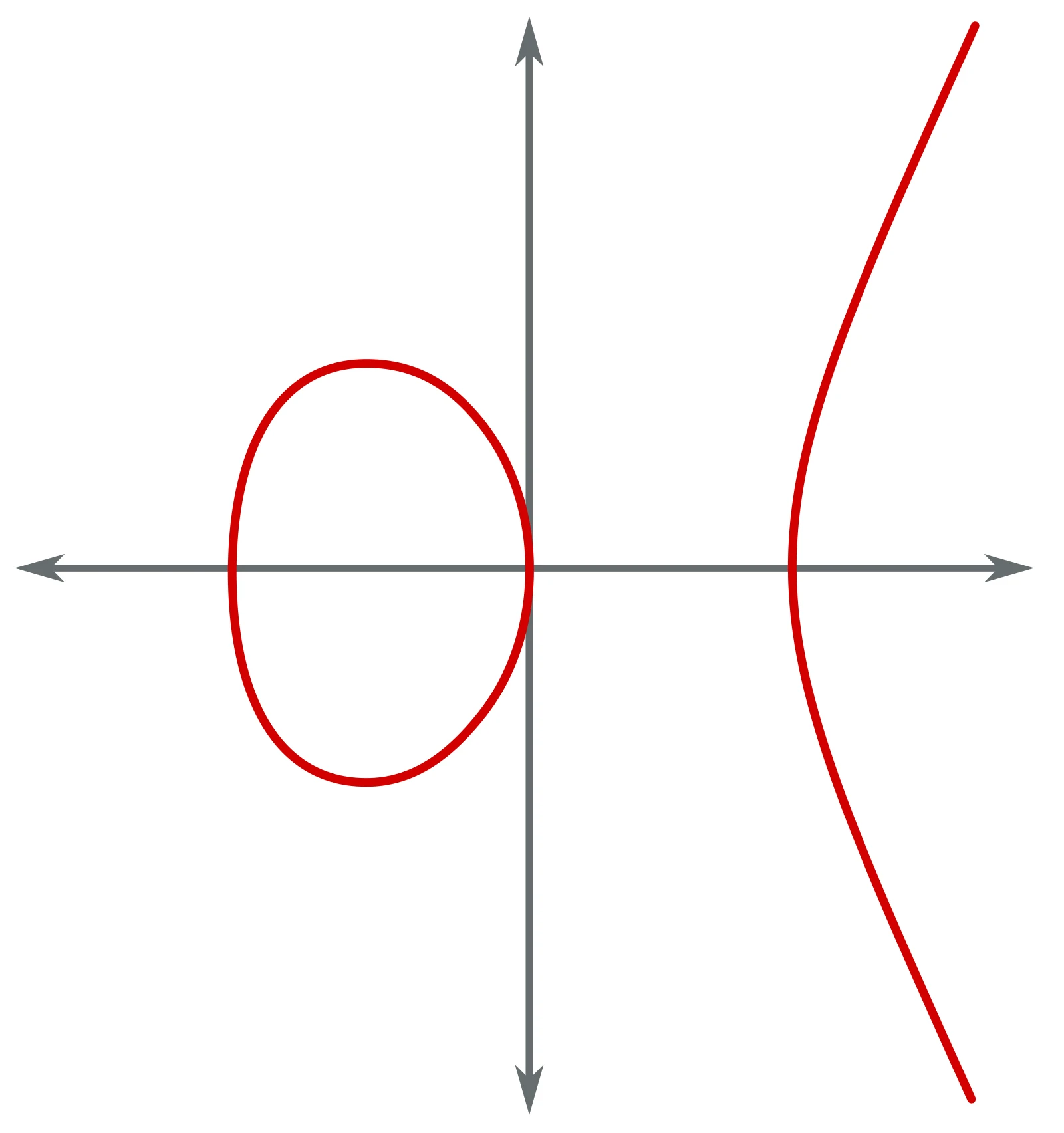
The Tate module of the elliptic curve already provided an ℓ-adic representation of Galois. Étale $H^1$ is closely related to its dual. This was a crucial precedent: ℓ-adic linear algebra was not invented from nothing for arbitrary varieties. Abelian varieties and their torsion points exhibited the coefficient tower in a classical setting. Grothendieck’s program sought a cohomology that placed this example beside all smooth projective varieties.

Higher dimensions multiply the middle degrees. For a smooth projective surface, degrees zero through four can contribute. Algebraic cycles appear naturally in even degrees, and the middle degree can carry classes not visibly generated by cycles. Duality pairs degree $i$ with $2d-i$, while weights should place eigenvalues on circles of radii $q^{i/2}$. The simple curve numerator becomes a layered factorization.

The examples show why “Betti numbers” and “Riemann hypothesis” were separate assertions. Knowing that $P_i$ has degree $b_i$ counts eigenvalues. It does not control their sizes. Knowing duality relates complementary products. It does not place each eigenvalue on the desired circle. The machine’s parts answered different clauses of the package.

Which Frobenius?

Over $\mathbf F_q$, the map on coordinates $x\mapsto x^q$ is often called arithmetic Frobenius in its action on an algebraic closure. The geometric Frobenius is the inverse automorphism. On schemes, an absolute or relative Frobenius map enters with another variance. Cohomology is contravariant for pullback, so the operator appearing in a trace formula depends on conventions.

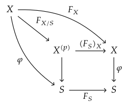
The distinction is not an antiquarian nuisance. If one operator has eigenvalue $\alpha$, its inverse has eigenvalue $\alpha^{-1}$. A determinant written as $\det(1-tF)$ changes accordingly, as does the statement of weight. Authors may place a power of $q$ or a reciprocal root on opposite sides while asserting the same geometry. A biography need not choose one notation for all sources, but a technical window must declare its choice. The trace and determinant displays in this chapter use geometric Frobenius.

The fixed-point relation provides the invariant core. Rational points over $\mathbf F_{q^n}$ are fixed by the appropriate $n$-fold Frobenius action on geometric points. The trace formula matches that action with the corresponding endomorphism on cohomology. Once the convention is fixed, the determinant identity follows consistently.

The semilinear origin of Frobenius also matters. It is not an arbitrary self-map selected to make a formula work. It comes from the finite field’s canonical endomorphism and commutes with algebraic structure. Its iteration corresponds exactly to extension from $\mathbf F_q$ to $\mathbf F_{q^n}$. This is why all point counts can be powers of one operator rather than unrelated measurements.

For a sheaf with Galois or monodromy action, local Frobenius at a closed point acts on a stalk after choosing a geometric point above it. Its conjugacy class is canonical under the usual conditions even when the chosen lift is not. Euler factors therefore depend on characteristic polynomials, which ignore conjugation. The same preference for invariant relational data appears again.

Ramified sheaves complicate local terms. Inertia groups, wild ramification, and conductors affect the L-function and functional equation. SGA 5’s title may sound as though one universal determinant handles everything without correction. The actual theory distinguishes lisse sheaves, constructible sheaves, and local behavior. The machine has settings.

This technical complexity is why the biography should avoid writing Frobenius as a personified agent that simply “revealed” hidden numbers. Frobenius action became useful because the categories, coefficient systems, and trace maps had been built so that its action was defined and calculable. Canonical arithmetic supplied the operator; collective geometry supplied the stage.

Local Euler factors, global determinants

For a constructible ℓ-adic sheaf $\mathcal F$ on a variety over $\mathbf F_q$, one can associate a local factor to each closed point $x$. The residue field at $x$ has size $q^{\deg x}$, and geometric Frobenius $\mathrm{Frob}_x$ acts on the inertia-invariant part of the geometric stalk; write the inertia group as $I_x$. A determinant $$\det(1-t^{\deg x}\mathrm{Frob}_x\mid \mathcal F_{\bar x}^{I_x})^{-1}$$ provides the standard local factor.

Multiplying these factors over all closed points gives an Euler product. Formally, taking logarithms expands the product into sums of traces of powers of local Frobenius. Closed points of degrees dividing $n$ combine to count rational points over $\mathbf F_{q^n}$, weighted by traces on stalks. The local product and the extension-field series are two organizations of the same arithmetic data.

The global trace formula then expresses that Euler product as an alternating product of determinants on $H^i_c(X_{\bar{\mathbf F}_q},\mathcal F)$. The local-to-global passage is not a coincidence. A sheaf binds the stalks through monodromy; cohomology measures the global organization. L-functions thus become a test of whether sheaf theory has captured arithmetic variation.

For the constant sheaf, the local trace is one and the L-function is the zeta function. For a sheaf arising from a representation, local traces can encode much richer sequences. This enlargement was one reason the cohomological explanation surpassed a proof of rationality for constant coefficients. The machine could accept coefficient objects as part of its input.

The Euler product also connected algebraic geometry with analytic number theory. One writes a formal or complex variable and asks about poles, zeros, and functional equations. Yet the cohomological determinant is algebraic. It identifies factors with characteristic polynomials of Frobenius. Analysis, arithmetic, and geometry meet without becoming the same discipline.

The passage required constructibility and finiteness. A sheaf varying arbitrarily could produce infinite-dimensional cohomology or uncontrolled local factors. Constructible sheaves are locally finite in a stratified sense. They made it possible to enlarge coefficients beyond local systems while retaining a finite machine. The definition’s technical appearance records the boundary between portable variation and chaos.

By 1966, not every later theorem about general ℓ-adic sheaves, ramification, and independence of $\ell$ had been settled. The program’s direction was clear; its full modern category was not. This is precisely where the 1977 redaction cannot be read without historical caution. The mature book is evidence of what the program became.

Compact support and the boundary

Ordinary cohomology behaves best for proper varieties, the algebraic analogue of compact spaces. If $X$ is not proper, a compactification $j:X\hookrightarrow\bar X$ places it inside a proper scheme with boundary. Extending a sheaf by zero and taking cohomology on $\bar X$ gives the model for compactly supported cohomology. The result must be shown independent of suitable choices.

This construction explains why a boundary cannot be ignored. Rational points live in $X$, not in an arbitrary compactification. Extension by zero prevents boundary sections from being counted as interior data. At the same time, exact sequences relating an open part and its closed complement allow cohomology to be assembled. The machine controls subtraction through distinguished triangles or long exact sequences.

Additivity is central to point counting. If $X$ is decomposed into a closed subscheme $Z$ and open complement $U$, then $\#X(\mathbf F_{q^n})=\#Z(\mathbf F_{q^n})+\#U(\mathbf F_{q^n})$. Compactly supported cohomology has a corresponding long exact sequence, so alternating traces add. The geometric decomposition and the linear-algebraic decomposition match.

Correspondences generalize maps. A cycle in $X\times X$ can define an action on cohomology, and its intersection with the diagonal supplies fixed-point data. Frobenius itself can be represented through its graph. The Lefschetz formula is therefore entangled with intersection theory, explaining why SGA 5 leads naturally toward the SGA 6 program beginning in 1966–67.

Nontransverse intersections produce local multiplicities. Counting visible fixed points with coefficient one would be wrong. The trace formula must match scheme-theoretic intersection numbers under appropriate conditions. This is another place where nilpotents and infinitesimal structure matter to a numerical output.

The boundary and local-term issues show that “count points by traces” is not one stroke of insight. It is a compatibility between two additive formalisms: scheme-theoretic decomposition and derived cohomology. Each exceptional case teaches the architecture which functor or correction it lacks.

Grothendieck’s method accepted the expansion. Rather than reserve the theorem for smooth projective varieties, the program sought compact support and constructibility so singular or open schemes could enter. Generality increased the technical burden but made the resulting trace formula a reusable instrument.

A family crossing characteristics

Suppose a smooth proper variety in characteristic $p$ is the special fiber of a smooth proper scheme over a discrete valuation ring whose generic fiber has characteristic zero. After choosing $\ell\ne p$, smooth and proper base change can relate the ℓ-adic cohomology of the geometric fibers. If the generic fiber embeds into $\mathbf C$, comparison can relate its étale cohomology to singular cohomology. This route imports Betti numbers without importing complex points into the special fiber.

Every clause in that sentence does work. A lift to characteristic zero need not exist. Smoothness and properness may fail. The residue and fraction fields require geometric closures. Comparison uses finite or ℓ-adic coefficients in a controlled way. The conclusion is not that the two fibers are the same space; it is that their cohomology belongs to one compatible sheaf-theoretic family.

Varieties that do not lift cannot be excluded from Weil’s conjectures. The general theory therefore needed arguments independent of lifting, along with spreading-out and alteration techniques developed over time. The lifting picture explains the desired answer but does not prove it for all cases.

This limitation helps explain Grothendieck’s interest in algebraic cycles and motives. If different cohomology theories share formal properties and agree on cycles, perhaps they are realizations of a more universal object. Such an object could explain independence of the auxiliary prime and carry weights intrinsically. In the middle 1960s this was a program, not a completed category with every desired property.

The relative base made the question possible. Instead of comparing two unrelated varieties in different characteristics, one studies fibers of one morphism. Specialization, nearby cycles in later form, and monodromy become relations inside a family. The scheme-theoretic foundation again turns a philosophical analogy into a map.

The family view also reshaped arithmetic reduction. A variety over a number field can be spread out over an open part of the spectrum of its integers. Each prime of good reduction supplies a finite-field fiber and a Frobenius polynomial. Global arithmetic can be assembled from these local fibers. Étale cohomology provides the representations on which all those Frobenius elements act.

Not all of this global theory was complete in 1966. The architecture made its questions legible. That is the historical point: a framework can alter mathematical practice before every intended comparison becomes a theorem.

Cycles, positivity, and the later conjectures

Algebraic cycles—formal combinations of subvarieties—act on cohomology through their classes. Intersections of cycles produce pairings. In classical complex geometry, Hodge theory supplies strong positivity and decomposition results. Over finite fields, an analogous algebraic control of cycles might constrain Frobenius eigenvalues.

This hope led Grothendieck toward motives: a universal layer of geometry from which different cohomology theories would arise as realizations. The word motive belongs to the middle of the decade in correspondence and discussion, but its exact technical meanings evolved. Chapter 38 will address the program directly. Here it should appear only as the horizon opened by the ℓ-dependence and weight problems.

The standard conjectures on algebraic cycles later proposed hard Lefschetz and positivity statements in an algebraic form. If true, they would yield major parts of the Weil package through a Weil cohomology. But the printed statement used for this account comes from the 1968 Bombay meeting and 1969 publication. It cannot be inserted as a theorem or finished plan of the 1965–66 seminar.1515Grothendieck, “Standard Conjectures on Algebraic Cycles”.

Tate’s 1965 conjecture took another route: poles of zeta functions, or equivalently fixed subspaces for Frobenius after a twist, should measure algebraic cycles of a given codimension. It connected observable arithmetic behavior to the elusive algebraic classes. The conjecture was neither a corollary of SGA 5 nor a duplicate of Grothendieck’s later standard conjectures.1616Tate, “Algebraic Cycles and Poles of Zeta Functions”.

These programs exposed a surprising inversion. Cohomology had been invented to explain zeta functions, yet zeta functions could now be used to predict which cohomology classes were algebraic. Arithmetic output interrogated the machine’s internal geometry. The relation ran both ways.

Positivity was the stubborn part because category-theoretic functoriality does not impose an inequality on complex absolute values. One needs a form, pairing, or geometric argument strong enough to constrain spectra. This is why the rising architecture stopped at the wall of weights. More formal reach did not automatically produce order.

Deligne’s later proof found a route through the behavior of sheaves in families, monodromy, and induction rather than by first proving all standard conjectures. That later success demonstrates that Grothendieck’s proposed road was not the only one. It also demonstrates the power of the SGA architecture Deligne inherited and reshaped. Both facts must coexist.

The state of the program at the end of 1966

The state of the program can be divided into records rather than compressed into the word “solved.” Dwork’s rationality theorem was published in 1960. The SGA 4 seminar of 1963–64 had developed the étale and topos foundations, though its revised volumes would not appear until 1972–73. Grothendieck’s Lefschetz-and-L-functions exposé belonged to 1964–65 and was printed in 1966. SGA 5 ran in 1965–66 and would be published only in 1977.

On the theorem side, substantial finiteness, comparison, base-change, duality, and trace machinery existed or was being established in the network. Exactly which version was proved by which date requires fascicle-level work. The revised books cannot settle that fine question alone. This account therefore describes the architecture and dates only claims anchored to contemporary publications or seminar labels.

On the conjectural side, the general absolute-value assertion remained open. Independence questions and cycle conjectures remained. A universal motives theory was not a completed replacement. The word “program” is not a polite synonym for theorem. It names a directed set of constructions and obstacles.

On the institutional side, the machinery had become collective. SGA 4’s direction was shared; SGA 5’s exposés had authors; EGA foundations were co-produced with Dieudonné; Harvard notes and seminars formed parallel channels. Grothendieck’s intellectual leadership is clearest when the network is visible, because the architecture coordinated work no single paper could contain.

On the biographical side, Grothendieck was thirty-eight. International recognition was imminent, but no document supports an image of him waiting for a verdict on a finished system. The mathematics in print during 1966 includes EGA IV.3, the algebraic de Rham paper, Hartshorne’s duality volume, and the Bourbaki exposé. Work and redaction continued on several fronts.

This audit prevents the Fields Medal from becoming a retrospective seal on Deligne’s future proof. The medal citation named achievements already recognized. It did not certify every aspiration. The distinction honors the open problem and the mathematician who later solved it.

The axiomatic shape of a Weil cohomology

Before étale cohomology could be judged, the desired formal properties had to be named. A Weil cohomology for smooth projective varieties should assign finite-dimensional graded vector spaces, be contravariantly functorial, possess cup products and Künneth isomorphisms, carry cycle-class maps, satisfy Poincaré duality, and provide a trace in top degree. Different later formulations arrange the axioms differently, but the architecture was already guiding the program.

Finite dimensionality turns traces and determinants into finite algebra. Künneth relates the cohomology of a product to tensor products and makes correspondences act. Cycle classes translate subvarieties into cohomological operators. Duality turns intersection pairings into perfect linear pairings. Together these properties make the Lefschetz number of a correspondence meaningful.

The axioms separated formal consequences from the construction of a theory. If any cohomology satisfied them and admitted Frobenius, portions of the Weil conjectures would follow by arguments independent of how the groups were built. Étale cohomology’s task was then twofold: exist over finite fields and verify the axioms in the necessary form.

This distinction was methodologically powerful. One could identify a missing axiom rather than say the whole theory “did not work.” If Künneth or duality was available but positivity was absent, the weight problem was isolated. If finite dimensionality failed for unrestricted coefficients, one changed the coefficient category.

The word machine is most accurate at this axiomatic level. A machine is not the material of one gear; it is the reliable composition of operations. Different cohomology theories can realize similar interfaces. The prospect of motives arose partly from asking what common source made those interfaces agree.

But the polished phrase “Weil cohomology” is itself later systematization. A historical chapter should not claim that one definitive axiom sheet governed every 1961 decision. The 1958 address, SGA programs, and later formulations show an evolving specification. Requirements became clearer as constructions were tested.

Correspondences turn geometry into operators

A morphism $f:X\to Y$ gives pullback on cohomology. A correspondence is more general: an algebraic cycle on $X\times Y$ can, using pullback, cup product with its class, and pushforward, define a map from cohomology of $X$ to cohomology of $Y$. This makes algebraic relations act linearly even when no ordinary function connects the spaces.

The graph of a morphism is a correspondence. Its intersection with the diagonal records fixed points. The trace of the induced operator should equal an intersection number. This is the geometric core of the Lefschetz formula and the reason intersection theory lies beside cohomology in the architecture.

Composing correspondences corresponds, under the right hypotheses, to composing operators. Fiber products and proper pushforward control the composition. The formula is another test of functorial compatibility: cycle classes must respect products, pullback, and pushforward or the operator calculus fails.

Frobenius has a graph, and its $n$-th iterate has fixed points defined over $\mathbf F_{q^n}$. The point-count problem therefore becomes an intersection between the graph of Frobenius and the diagonal. If the intersection is transverse, each point contributes simply; in general local terms carry multiplicity.

This formulation shows why algebraic cycles entered the route to weights. Beyond labeling known subvarieties, they are the geometric operators through which Frobenius and duality speak to cohomology. Understanding positivity of their pairings could constrain eigenvalues.

It also clarifies credit. Grothendieck’s architecture assembled cycle classes, duality, and correspondences, but intersection theory had a long history and SGA 5 exposés had individual authors. “Grothendieck–Lefschetz trace formula” is a standard name, not permission to remove that genealogy.

Finiteness is a theorem

The determinant formula silently assumes that each relevant cohomology group is finite-dimensional over $\mathbf Q_\ell$. For a finite-type scheme and a constructible torsion sheaf with torsion prime to the characteristic, finiteness theorems supply the needed control under standard hypotheses. These results are among the least glamorous and most load-bearing parts of the machine.

Without finiteness, one could still form cohomology groups, but traces might be undefined and characteristic polynomials infinite. Rationality would not follow. The passage from local finite data to global finite groups is therefore as essential as the fixed-point idea.

Constructibility is the coefficient-side hypothesis. A constructible sheaf becomes finite locally constant on each member of a finite stratification. It may have singular behavior along a boundary, but that behavior is controlled. This allows the theory to include extensions by zero and direct images without admitting arbitrary infinite variation.

Cohomological dimension bounds are another form of finiteness. They say that cohomology vanishes above degrees related to the dimension of the scheme under the appropriate conditions. A determinant product then has finitely many nontrivial degrees. The topological expectation that a $d$-dimensional smooth variety has cohomology only through degree $2d$ acquires an algebraic analogue.

Proving such statements often required induction on dimension, alterations of the space, local acyclicity, and reductions that are invisible in the final zeta formula. The machine’s elegance rests on a vast supply chain of estimates.

This labor also shaped SGA’s collective form. Finiteness and base change are too large to remain lemmas inside one point-counting paper. They became exposés and theories reusable far beyond the original application. A program converts a technical prerequisite into common infrastructure.

Independence of the auxiliary prime

Choose $\ell\ne p$ and the machine produces $\mathbf Q_\ell$-vector spaces. Choose another prime $\ell'\ne p$ and it produces different coefficient fields. The zeta function computed from traces is the same rational function with integer data. This forces characteristic polynomials of Frobenius to exhibit compatibility not visible from either construction alone.

For smooth proper varieties, the expected dimensions should be independent of $\ell$ and agree with Betti numbers when comparison is available. Traces of Frobenius powers, because they count points, are integers independent of $\ell$. Recovering individual characteristic polynomials from those traces gives important independence in favorable cases.

Yet “étale cohomology is independent of $\ell$” is too broad. Vector spaces over different fields cannot be canonically identified in a naive way. Independence may refer to dimensions, characteristic polynomials, compatible systems, or cycle classes. Each is a theorem or conjecture with hypotheses.

The auxiliary-prime problem drove the idea of a common motivic source. If several realizations produce compatible spectra, perhaps the geometry contains an object before coefficients are chosen. This philosophical inference was powerful because it arose from exact numerical coincidences.

In 1966 the full modern theory of compatible systems was not in place. The chapter therefore describes independence as a demand and partial achievement, not as a single settled theorem. Later results cannot be smuggled into SGA 5 through the notation $\ell$.

The issue also reveals why $p$-adic cohomology was needed. Excluding $\ell=p$ leaves the prime most intimately tied to the ground field outside the étale tower. Crystalline and later rigid cohomology would answer different parts of that need. Their later success confirms the plural architecture; it was not already available in the 1965–66 seminar.

Derived operations behind one product

The determinant formula uses compactly supported global cohomology, written $R\Gamma_c$ at the derived level. Constructing it typically involves an open immersion into a compactification, extension by zero, and ordinary derived global sections. Independence from compactification requires comparison maps and proper base change.

Tensor product enters because coefficient sheaves combine and cup products land in tensor products. Derived tensor product is needed when ordinary tensoring loses exactness. Internal derived Hom enters duality. Pullback and direct image transport coefficients along maps. Exceptional operations handle support and duality.

Each operation comes with adjunctions and natural transformations. A base-change square produces a map between pull-then-push and push-then-pull. A projection formula compares pushing a tensor product with tensoring a pushforward. Duality identifies an exceptional inverse image as an adjoint. These relations make the operations a formalism rather than a list.

The phrase “six functors” can make the system sound finished by 1966. It was not finished in every later generality. Different categories of sheaves and maps required continuing work. What existed was a powerful direction and major pieces sufficient to formulate trace and duality results.

Verdier’s derived methods were crucial because adjunctions and triangles retain information lost when one takes cohomology groups too early. A long exact sequence is the shadow of a distinguished triangle. The global trace formula is easier to make additive when the derived object itself is additive.

Grothendieck’s architectural instinct appears here as insistence on compatibility before calculation. One can compute a zeta function in examples without six operations. One cannot build a theory that transports the calculation through open and closed decompositions, families, and sheaf coefficients without them.

The 1977 volume and the 1966 seminar

The title page of SGA 5 fixes two facts: the seminar belongs to 1965–66, and the Lecture Notes volume was published in 1977. Luc Illusie’s editorial role belongs to the latter object. A historian must resist turning the neat 1977 volume into a calendar for the earlier year.

Between those dates Deligne proved the Riemann-hypothesis component, SGA 4 appeared, and the field’s derived and ℓ-adic languages matured. An editor preparing SGA 5 could not unknow these developments. Revisions might clarify statements or mark gaps visible only later. The final volume is mathematically primary and chronologically layered.

Original fascicles would allow a finer map: which exposé circulated when, what corrections entered, and which theorems were complete at the seminar’s end. This account does not claim to have completed that fascicle consultation. It therefore uses the 1966 Bourbaki exposé as a contemporary public statement and the 1977 volume for the mature architecture.

The distinction changes verbs. “In 1965–66 the seminar pursued ℓ-adic cohomology and L-functions” is secure. “SGA 5, published in 1977, proves” describes the book. “By June 1966 Grothendieck’s group possessed the final proof of exposé X” requires additional dated evidence. The prose avoids the third form.

Publication delay also complicates influence. A mathematician could learn the results from notes or people before 1977. Another could independently develop a method because the book was inaccessible. Citation history cannot be read from the imprint alone. The network distributed knowledge unevenly.

This is not a defect unique to SGA. Research often precedes definitive publication. SGA makes the distance unusually large and the later authority unusually strong. That combination demands unusually explicit chronology.

What the machine changed outside the conjecture

Even before the general weight theorem, étale cohomology transformed the arithmetic study of varieties. Fundamental groups encoded finite covers; Galois representations arose from cohomology; torsion in Picard and Brauer groups became accessible; base change controlled families. These uses did not wait for the full Weil package.

The theory also connected local fields and global varieties. Inertia and ramification acted on stalks and cohomology. Specialization maps compared fibers. Monodromy recorded degeneration. L-functions attached to sheaves provided a common language for many arithmetic generating series.

Some of the most celebrated later applications lie far beyond 1966 and should not be listed as if they motivated SGA 5. Their relevance is evidentiary: the interfaces proved portable. A tool built for one horizon became infrastructure for another.

This portability explains why an unfinished machine could revolutionize a field. Its value was not binary, equal to zero until the last conjecture fell. Every verified operation changed which questions could be asked and how answers traveled.

Grothendieck’s program thus altered mathematical temporality. A major theory could be worth building before the motivating theorem was secured because its intermediate objects had independent lives. The risk was justified by surplus.

The same fact made later credit complex. Users could extend the theory in directions Grothendieck did not pursue. Their results belong to them even when the language belongs to his school. Infrastructure creates common property while retaining specific invention.

Recovering a polynomial from its traces

The determinant identity has an elementary linear-algebra counterpart. If an operator $T$ on a finite-dimensional vector space has eigenvalues $\alpha_1,\ldots,\alpha_m$, then $\operatorname{Tr}(T^n)=\sum_j\alpha_j^n$. The sequence of power sums determines the characteristic polynomial through Newton identities. Infinitely many traces are constrained by finitely many coefficients.

Point counts supply alternating sums of these traces across cohomological degrees. The known contributions in degrees zero and top degree can sometimes be separated, leaving a middle polynomial. For curves, the first several counts determine the zeta numerator. The machine predicts recurrences among all later counts.

Rationality is therefore a finite-memory statement. The sequence $N_n$ may look like new arithmetic information at every extension degree, but cohomology says it comes from powers of finitely many eigenvalues. A rational generating function and a linear recurrence are two forms of the same compression.

Weights add an analytic constraint to this algebraic compression. They do not change the recurrence; they bound the size of its terms and hence the error in point counts. This is why rationality could be proved while the Riemann hypothesis remained open. Finite memory does not determine spectral radius.

The example also explains why traces alone can conceal degree-by-degree information. Alternating sums permit cancellation. Künneth, duality, and comparison help identify which eigenvalues belong to which cohomological degree. The full architecture decomposes what one numerical sequence combines.

Two kinds of explanation

Dwork’s proof and the cohomological proof should not be arranged as an inferior calculation followed by a superior concept. A direct method can reveal structures the general framework misses; a framework can explain relations a direct proof does not address. Mathematics advances by both.

The p-adic route worked close to the characteristic and developed analytic operators suited to point counting. The ℓ-adic route deliberately chose $\ell\ne p$ and constructed topological-style cohomology. Their contrast showed that a theorem can have several reasons.

For Grothendieck, the cohomological reason mattered because Weil’s assertions formed a package. Rationality, functional equation, Betti degrees, and weights resembled formal consequences of topology plus positivity. A proof of one clause did not make the package accidental.

For a historian, Dwork’s priority is nonnegotiable and Grothendieck’s explanatory ambition is also nonnegotiable. Erasing the first creates false credit; erasing the second makes SGA’s scale unintelligible. The notes keep the 1960 paper and the 1964–66 program beside one another.

The coexistence is a lesson in plural cohomology. Later p-adic theories would provide their own geometric realizations, while ℓ-adic theory would dominate other applications. No one coefficient field held a monopoly on explanation.

The open problem as a transfer of agency

Once the weight problem had been isolated, it became available to other mathematicians in a sharper form. They did not need to rebuild schemes, sites, and trace formulas before asking how eigenvalues were constrained. Infrastructure transferred agency to the next investigator.

That transfer is one reason the architecture should not be described as Grothendieck’s private machine. It was published, taught, and revised so others could operate and modify it. Deligne’s later theorem exemplified the transfer but was not its predetermined output.

An open problem inside a mature language differs from a vague mystery. Examples, functorial operations, and partial theorems specify what a solution must respect. The language can rule out false shortcuts and make analogies with monodromy or families precise.

Grothendieck’s achievement in 1966 included this redistribution. He had not solved the general Riemann hypothesis, but he helped make its next form possible. The distinction between solving and enabling is not a consolation prize; it is a different historical claim with different evidence.

What rationality does not say

A rational zeta function can have reciprocal roots of many complex sizes. Rationality says the point-count sequence satisfies a finite recurrence; it does not say the recurrence has the geometric balance predicted by weights. Functional equation adds symmetry but still need not place every root on the required circle.

Likewise, the degree of a factor can match a Betti number while its eigenvalues have the wrong magnitude. The four parts of Weil’s package reinforce one another without being logically identical. A proof of one must not be narrated as a blurred proof of all.

This separation explains the research sequence. Dwork could settle rationality before étale cohomology matured. Duality could account for reciprocal symmetry. Comparison and base change could identify dimensions. The weight theorem required a further argument.

The machine’s value was partly diagnostic. It assigned each observed regularity to a structural source and displayed the clause for which no source was yet adequate. An open conjecture became a missing mechanism.

That diagnosis also protected future credit. When Deligne supplied the weight argument, his theorem had a clearly delimited content. The architecture explained why it completed the package; it did not make the completion automatic.

A machine with a horizon

The cohomological machine did not face a finite list of inputs known in advance. Every new sheaf, family, or singularity tested its interfaces. Its horizon moved as soon as one theorem worked. Rationality led to L-functions with coefficients; duality led to exceptional operations; comparison led to independence questions.

This expansion distinguishes architecture from a trick. A trick may solve one problem brilliantly and end there. An architecture exposes adjacent problems and gives them common notation. Its success increases rather than decreases the amount of visible unfinished work.

By 1966 Grothendieck had built such visibility. The open weight problem stood among proven constructions rather than in an unstructured field of questions. That is why the program could be both incomplete and already consequential.

The affine line and compact support

The affine line supplies a compact-support check that differs from the projective line. For every $n$, $$\#\mathbf A^1(\mathbf F_{q^n})=q^n,$$ so its zeta function is $1/(1-qt)$. The missing factor $1/(1-t)$ reflects the missing point at infinity.1717Weil, “Numbers of Solutions of Equations in Finite Fields”; Milne, Étale Cohomology.

Ordinary cohomology alone does not express this count in the desired alternating form. For $\ell\ne p$, $H_c^2(\mathbf A^1_{\overline{\mathbf F}_q},\mathbf Q_\ell)\cong \mathbf Q_\ell(-1)$. With geometric Frobenius acting on $\mathbf Q_\ell(-1)$ by $q$, its $n$-th power has trace $q^n$. The subscript $c$ records the boundary condition rather than a cosmetic variant.1818Illusie, Cohomologie ℓ-adique et fonctions L (SGA 5); Grothendieck, “Formule de Lefschetz et rationalité des fonctions L”; Milne, Étale Cohomology.

Embedding $\mathbf A^1$ into $\mathbf P^1$ makes additivity visible: the projective line is the disjoint union of the affine line and the point at infinity. Point counts add, and the long exact sequence for compact supports produces the corresponding alternating trace relation.1919Illusie, Cohomologie ℓ-adique et fonctions L (SGA 5); Milne, Étale Cohomology.

The example also gives a boundary to the machine analogy. A determinant formula does not choose the correct cohomology automatically. The open variety forces a theory of supports, extension by zero, and independence from compactification. Each operation requires a theorem.

Historically, such examples justified the expansion beyond smooth projective varieties. SGA 5 needed L-functions for sheaves and nonproper spaces, not only the case in which ordinary cohomology already resembled compact topology. The arithmetic target made compact support part of the program.2020Illusie, Cohomologie ℓ-adique et fonctions L (SGA 5); Grothendieck, “Formule de Lefschetz et rationalité des fonctions L”.

The affine-line computation is elementary only after the correct cohomology has been chosen. Before that choice, the missing point at infinity creates the discrepancy between ordinary and compactly supported behavior. The example therefore tests the formalism rather than decorating it.

It also keeps the chronology exact. The trace program’s historical importance lies in connecting such computations through a reusable theory, not in claiming that every zeta function first became rational through étale cohomology. Dwork’s 1960 proof retains its distinct priority.2121Dwork, “On the Rationality of the Zeta Function of an Algebraic Variety”; Grothendieck, “Formule de Lefschetz et rationalité des fonctions L”.

In this form, the example completes the explanatory circuit: a counting problem leads to a concrete variety, the trace formula supplies the precise kernel, compact support gives the computation, the missing boundary point identifies the limit, and SGA 5 provides the historical return to Grothendieck’s program.

Explanation without completion

By the end of 1966, the cohomological vision had changed the Weil problem. Point counts could be sought as Frobenius traces. Zeta functions could be expressed through determinants. Functional equations could be linked to duality. Betti-number behavior could be approached through comparison and base change. The hardest weight estimate remained open.

This state resists the usual narrative shape. A biography likes a problem, a period of struggle, and a solution crowned by a prize. Here the prize arrived before the general solution, and the eventual proof belonged to a younger collaborator using tools the program had made available. The more faithful shape is architectural: foundations, a functioning wing, an unfinished span, and work continuing through the ceremony.

The program’s methodological achievement was to make incompletion informative. The machine did not stop at failing to prove the Riemann hypothesis. It translated the failure into a question about eigenvalues, cycles, and positivity. It showed that rationality and duality belonged to formal cohomological structure while weights required a further idea. The boundary became a research program.

This is the opposite of a magical abstraction that dissolves every problem. The general language succeeded because it could reveal where formalism stopped. A category, site, or functor is not an answer by prestige. It earns its place through theorems, and the absence of a theorem remains visible.

In August 1966, the Fields Medal recognized Grothendieck’s existing body of work. The IMU summary emphasized algebraic geometry, K-theory, and the Tôhoku paper rather than claim a completed Weil proof. The cohomological program formed part of the work recognized, while the weight problem remained open.2222International Mathematical Union, “Fields Medals 1966,” https://www.mathunion.org/imu-awards/fields-medal/fields-medals-1966.

The trace formalism depended on named collaborators who proved, transmitted, and edited its components. Their distinct roles and routes through Harvard and Paris lead directly to the documentary network of Chapter 35. Collective labor was a condition of the mathematics, not background scenery.